


| Issue |
Int. J. Metrol. Qual. Eng.
Volume 17, 2026
|
|
|---|---|---|
| Article Number | 11 | |
| Number of page(s) | 18 | |
| DOI | https://doi.org/10.1051/ijmqe/2026009 | |
| Published online | 18 June 2026 | |
Research Article
A graph-aware meta network for domain generalization in cross-condition bearing RUL prediction
1
Guangxi Zhuang Autonomous Region Toll Highway Network Toll Collection Clearing and Settlement Center, PR China
2
Guangxi Transportation Science and Technology Group CO., LTD., PR China
* Corresponding author: This email address is being protected from spambots. You need JavaScript enabled to view it.
Received:
7
March
2026
Accepted:
19
May
2026
Abstract
Driven by advances in sensor technology, data-driven remaining useful life (RUL) prediction has become an important tool for bearing predictive maintenance. However, variations in operating conditions in industrial applications can cause feature distribution shifts, thereby reducing the accuracy and robustness of prediction models. To address feature distribution shifts across operating conditions, this paper proposes a graph-aware meta network based on domain generalization for bearing RUL prediction across conditions. The proposed method converts monitoring sequences into graph structured inputs and employs a temporal encoder to learn node-level degradation representations. It further integrates prior structural knowledge, globally shared structure, and task-adaptive structure to build multi-level dynamic adjacency relationships, and introduces an attention pooling mechanism to obtain graph-level degradation representations. During training, a meta-learning strategy with inner and outer loop updates is designed to dynamically adapt the graph generation parameters, enabling task-specific topology to adjust automatically with changing operating conditions and thereby improving model generalization. Cross-condition experiments on a public bearing accelerated life dataset demonstrate that the proposed method achieves superior prediction error metrics across multiple transfer tasks and delivers stable performance under varying operating conditions.
Key words: Remaining useful life prediction / bearing / domain generalization / meta-learning / graph neural network
© Z. Wu et al., Published by EDP Sciences, 2026
 This is an Open Access article distributed under the terms of the Creative Commons Attribution License (https://creativecommons.org/licenses/by/4.0), which permits unrestricted use, distribution, and reproduction in any medium, provided the original work is properly cited.
1 Introduction
With the advancement of high-end equipment manufacturing and intelligent operation and maintenance (O&M), sensor-based condition monitoring and health management have become a critical technical approach to ensuring the safe and reliable operation of key rotating machinery [1–4]. Bearings, as one of the most essential and failure-prone components in rotating systems, are widely used in computer numerical control machine tools, rail transit, aero-engines, and other equipment, and they often operate under complex working conditions for extended periods [5–7]. If bearing faults are not handled in a timely manner, they may lead to performance degradation of the equipment in mild cases, and in severe cases can trigger cascading shutdowns or even safety accidents, resulting in substantial maintenance costs and production losses. Compared with corrective maintenance or fixed-interval overhaul, evaluating degradation states using online monitoring data and predicting the remaining useful life (RUL) allow maintenance and replacement strategies to be scheduled within a more appropriate time window, thereby optimizing maintenance resource allocation and reducing life-cycle costs [8–10].
However, during service, bearings are subject to coupled mechanisms involving wear, fatigue, and material degradation, and their degradation often exhibits strong nonlinearity and stage-wise characteristics. In the early stage, degradation typically manifests as weak and intermittent vibration variations, which then gradually evolve into more pronounced impulsive signatures and energy-concentration phenomena [11,12]. Owing to the pronounced nonlinearity and individual variability of the degradation process, even bearings of the same type may present different degradation trajectories under varying rotational speeds, loads, and lubrication conditions. In addition, practical engineering environments commonly involve noise interference and differences in sensor installation, which alter the statistical properties of the monitored signals. As a result, RUL prediction must not only accurately characterize degradation trends but also remain robust to noise perturbations and changes in operating conditions. Meanwhile, in real industrial scenarios, acquiring life-cycle labels is time-consuming and costly, which further increases the difficulty of RUL modeling and evaluation [13,14]. Therefore, highly reliable RUL prediction under complex operating conditions is a key enabling component for predictive maintenance and optimized O&M decision-making.
Although predictive maintenance research has made substantial progress in recent years, bearing RUL prediction still faces multiple challenges in engineering applications [15–17]. Conventional physics-based modeling approaches rely on an accurate characterization of material properties, loading conditions, and degradation mechanisms; they typically require extensive prior knowledge and are built upon restrictive assumptions, and thus often struggle to remain reliable under complex and partially unobservable real-world operating conditions [18,19]. With the continuous improvement of sensor technologies and data acquisition systems, data-driven methods have gradually become the mainstream for bearing RUL prediction. Such methods can learn degradation patterns directly from monitoring data, reducing reliance on mechanistic modeling and demonstrating strong predictive potential. In particular, deep learning models have attracted widespread attention in recent years due to their end-to-end representation learning capability. For example, Jin et al. [20] proposed a dual-channel spline graph convolutional network that captures spatial correlations among features through global topological aggregation, thereby enhancing the modeling of continuous local feature variations. Yin et al. [21] developed an RUL prediction framework based on deep ensemble learning and error correction, and validated its performance advantages experimentally. To address the weak early-stage degradation trend, Pan et al. [22] constructed a cumulative feature model to improve life prediction accuracy. However, these approaches typically rest on a key implicit assumption: the training and test data are identically distributed. Once operating conditions change, the learned representations often fail to maintain stable performance in practical deployment [23,24]. In real industrial settings, factors such as rotational speed, load, and environmental disturbances inevitably fluctuate, substantially altering the statistical characteristics of vibration signals and the evolution law of degradation, thereby inducing a shift between the feature distribution learned during training and that encountered at deployment [25]. Existing studies have shown that even for the same type of bearing, changes in operating conditions alone can significantly increase prediction errors. The distribution mismatch caused by operating-condition variations has therefore become a critical bottleneck that hinders the engineering application of data-driven RUL prediction methods [26].
To address the distribution shift in cross-condition RUL prediction, researchers have proposed various transfer learning and domain adaptation methods that improve cross-domain predictive performance by reducing representation discrepancies among different operating conditions. For instance, Tian et al. [27] developed a gradient-based uncertainty-weighting strategy to enable RUL prediction under unseen operating conditions. Focusing on offline distribution drift, Mao et al. [28] introduced a Wiener-process-assisted incremental updating mechanism to enhance prediction capability across varying conditions. Liu et al. [29] proposed a few-shot transfer enhancement method with interpretable contributions to improve prediction performance when target-domain samples are limited. In recent years, related studies on bearing fault diagnosis have also increasingly focused on cross-operating-condition adaptation, limited-sample learning, confidence-aware decision making, and imbalanced-data modeling. For example, Men et al. [30] investigated unsupervised domain adaptation for bearing fault diagnosis under extremely sparse sample conditions based on twin data, while Men et al. [31] addressed railway freight car bearing fault diagnosis on imbalanced datasets using an improved ACWGAN. These studies indicate that improving model robustness under sparse, imbalanced, and distribution-shifted data has become an important research direction in intelligent bearing health monitoring.
Although these methods alleviate the performance degradation caused by operating-condition changes to some extent, several issues remain. Most existing studies mainly focus on fault classification, sample enhancement, or distribution alignment, whereas cross-condition RUL prediction requires continuous degradation trajectory modeling and stable regression generalization under unseen operating conditions. On the one hand, beyond temporal and spectral information, bearing vibration signals also contain structural relationships across different dimensions, which are crucial for modeling degradation evolution [32]. On the other hand, under cross-condition scenarios, the coupling relationships among monitoring variables may drift as operating conditions vary. If such changes are captured only through static information, the model’s ability to characterize structural variations will be constrained, thereby affecting the stability and reliability of cross-domain prediction.
To address the above issues, this paper proposes a domain-generalized graph-aware meta network (DG-MGNet) for cross-condition bearing RUL prediction. First, temporal monitoring samples are reconstructed into graph structured inputs, and node-level degradation representations are learned via a temporal encoder. At the structural level, prior structure, globally shared structure, and task-adaptive structure are integrated to construct multi-level dynamic adjacency relationships. Graph convolutions and attention pooling are then employed to obtain graph-level degradation representations for RUL regression. Furthermore, we introduce a meta-learning strategy during training that updates the model in an inner loop and an outer loop. This allows the task-specific topology to adapt quickly to changes in operating conditions, improving prediction stability and overall accuracy in cross-condition transfer. The main contributions of this work are as follows:
A multi-scale graph structure modeling approach is proposed. By jointly modeling and fusing prior structure, globally shared structure, and task-adaptive structure, the method captures inter-node correlations and multi-scale relational information, enhancing the model’s capability to represent complex degradation dependency patterns.
A meta-learning-based task topology update mechanism is designed. Through joint optimization in the inner and outer loops, task-relevant topology is dynamically updated in response to operating-condition variations, which improves transfer performance and stability in cross-condition prediction.
In what follows, Section II introduces the cross-condition task setting and the graph-based RUL prediction pipeline. Section III details the proposed DG-MGNet. Section IV reports experimental results, while Section V provides ablation and visualization analyses. Section VI concludes the paper and discusses future work.
2 Theoretical foundation
2.1 Cross-domain prediction
In cross-condition bearing RUL prediction, the source domain and the target domain usually correspond to different operating conditions, under which the vibration-signal distribution and degradation evolution can differ substantially. Let the source-domain vibration time-series dataset be  , where each sample
  is a vibration segment composed of T consecutive time points, and the corresponding RUL label set is denoted as
  . The target-domain vibration dataset is denoted as
  , whose data distribution differs from that of the source domain, as expressed in equation (1):
 (1)
(1)
where ps(x) denotes the feature distribution of the source domain, and pt(x) denotes the feature distribution of the target domain.
The distribution discrepancy mainly arises from variations in operating conditions, such as differences in rotational speed, load, or environmental factors. In practical scenarios, target-domain samples often lack life labels or contain only a small amount of labeled data, making it difficult to perform supervised learning directly on the target domain. Under this setting, the goal of cross-condition bearing RUL prediction is to learn a prediction model from labeled source-domain data that can generalize to the target operating condition. Specifically, this objective can be formulated as a regularized optimization problem, as shown in equation (2):
 (2)
(2)
where φ(·) denotes the learnable feature mapping; fθ(·) is the RUL prediction function;  represents the distribution discrepancy between source- and target-domain representations, and λd is the corresponding regularization weight.
2.2 Graph-based bearing RUL prediction
The graph convolutional neural network (GCN) can perform representation learning on non-Euclidean structured data and achieve information fusion by modeling the relationships between nodes. In GCN-based bearing RUL prediction methods, raw monitoring data must be preprocessed and converted into graph structured data as the network input to perform the RUL prediction task.
As shown in Figure 1c, a graph structured sample G = (V, E, X) consists of three core components: a node set  representing data entities, an edge set
  describing the relationships among nodes, and a node feature matrix
  encoding the attributes of each entity. A GCN iteratively updates node features via neighborhood aggregation, which can be written as equation (3):
 (3)
(3)
where  is the normalized adjacency matrix, W(l) is a learnable parameter matrix, and
  denotes the activation function. Here,
  denotes the node feature matrix at the l th graph convolution layer, where N is the number of graph nodes and F is the feature dimension.
Compared with conventional time-series and sequence data, graph structured data are not restricted to Euclidean space and can flexibly represent topological relationships among nodes through the adjacency matrix  . This non-Euclidean property enables graphs to effectively uncover implicit coupling relationships among multi-scale monitoring signals. In the bearing RUL prediction task, the graph representation can be understood as an organized description of degradation-related monitoring information. For each sample window, degradation features extracted from vibration signals are arranged as graph nodes, and the adjacency matrix describes the relationships among these nodes. If two feature channels show correlated changes during degradation, the corresponding edge weight tends to be larger, allowing stronger information interaction during graph propagation.
The GCN operation therefore does not simply replace temporal modeling. Instead, it complements temporal feature extraction by modeling the coupling structure among different degradation descriptors. Through neighborhood aggregation, each node updates its representation using both its own degradation information and the information from related nodes. After several graph convolution layers, the updated node representations contain both local degradation trends and cross-feature dependency information, which can then be further pooled and mapped to the RUL output. Under this formulation, bearing RUL prediction can be expressed as learning a mapping function  , i.e., from graph data to the RUL space.
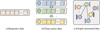 |
Fig. 1 Different types of monitoring data. |
3 Proposed method
To fully capture the multi-scale structural dependencies in bearing monitoring signals and to mitigate feature distribution shifts under cross-condition scenarios, we propose DG-MGNet. The key design motivations and implementation details of each module are presented in the following.
3.1 Multi-level graph structured degradation representation
Bearing monitoring signals often contain coupled degradation information, and the correlations among different feature dimensions may change as degradation progresses. By leveraging graph propagation, the proposed model enables cross-dimensional information interaction while preserving temporal characteristics, thereby improving the capability of modeling complex degradation behaviors.
From the physical perspective, the graph nodes in this study are not regarded as arbitrary mathematical variables. Instead, they are constructed from degradation-related vibration feature channels extracted from the horizontal and vertical acceleration signals. These features can be roughly associated with three types of degradation information: amplitude-energy features, such as standard deviation, RMS, peak-to-peak value, and band power, which reflect the increase of vibration intensity during bearing degradation; impact-sensitive statistical features, such as skewness and kurtosis, which are related to intermittent shocks caused by local defects; and frequency-domain features, such as median frequency, average frequency, maximum spectral amplitude, dominant frequency, and maximum power spectral density, which describe the redistribution and concentration of vibration energy in the frequency domain. Therefore, each node represents a local degradation descriptor or a physically related feature subset, while the graph topology describes the coupling relationships among these degradation descriptors.
Motivated by these advantages, we reconstruct the temporal vibration samples into graph data  and perform multi-scale graph-based degradation feature extraction, as illustrated in Figure 2. Specifically, the monitoring information is partitioned into F nodes, where each node corresponds to a subset of features. In this study, the node partitioning is performed according to the extracted feature channels and sensor directions. For each vibration segment, 14 time-domain and frequency-domain features are extracted from the horizontal acceleration signal, and the same 14 features are extracted from the vertical acceleration signal. Therefore, the graph contains F=28 nodes in total, and each node represents the temporal evolution of one specific degradation feature from one sensor direction. In this way, degradation information is decomposed into two parts: (i) the temporal degradation pattern within each node and (ii) the coupling structure among nodes.
The edge weight between two nodes characterizes the strength of degradation-related correlation between the corresponding feature channels. This correlation has a clear time-frequency interpretation. For example, when a local bearing defect gradually develops, impulsive responses in the time domain may become stronger, leading to simultaneous changes in RMS, peak-to-peak value, kurtosis, and spectral energy. Similarly, the propagation of defect-induced impacts through the rolling element-raceway-housing-sensor path may cause correlated responses between horizontal and vertical vibration features. Therefore, a large edge weight indicates that two feature channels jointly participate in describing the same degradation evolution or fault-propagation process.
For the local sequence xi of the i th node, a temporal encoder is used to extract the node embedding hi. Stacking the embeddings yields the node representation matrix  , which can be expressed as equation (4):
 (4)
(4)
where  denotes the temporal encoder composed of multiple 1D convolutional blocks to extract multi-scale degradation information within each node, and θt represents all learnable parameters of the temporal encoder.
To capture the drift of feature coupling relationships under varying operating conditions, a fused adjacency matrix is constructed by combining prior, global, and task-adaptive adjacency components, as shown in equation (5):
 (5)
(5)
where A0 is the prior adjacency matrix, which alleviates noise propagation caused by structural uncertainty in the early training stage; Ag is the global adjacency matrix that captures condition-invariant average coupling patterns across domains; Aθ is the task adjacency matrix that models structural drift for a specific source-to-target transfer task; and  denotes the Sigmoid activation function.
Considering that labeled data under the target condition are often scarce, the task structure Aτ should be inferred quickly from a small number of samples. To this end, we introduce a node-prototype-driven attention graph generation mechanism. Specifically, node prototypes  are obtained by mean aggregation over node embeddings, and the task adjacency matrix Aτ is then constructed by computing pairwise similarities among prototypes. The procedure is given in equations (6) and (7):
 (6)
(6)
 (7)
(7)
where Wq and Wk are learnable projection matrices; Q and K denote the query and key mappings, respectively; and √d is the scaling term.
Given the fused adjacency matrix Am, degradation propagation is modeled via graph message passing, as in equation (3). The graph convolution layer aggregates degradation representations from neighboring nodes according to the learned structure, thereby capturing the diffusion and transmission of degradation information over the coupled system.
To emphasize the contributions of informative nodes, an attention pooling module is employed to generate a graph-level representation, as expressed in equation (8):
 (8)
(8)
where αi denotes the importance weight of the i th node for prediction, hi is the final-layer node representation, q is a learnable attention query vector, and z denotes the graph-level embedding.
Finally, a regression head outputs the RUL prediction. The overall prediction function can be written as equation (9):
 (9)
(9)
where  denotes the regression head consisting of two MLP layers, θr are its parameters, θ denotes the set of all learnable parameters in the network, and Am is the fused adjacency matrix.
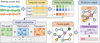 |
Fig. 2 Degradation feature extraction based on multi-scale graph. |
3.2 Meta-learning optimization strategy
A model trained under a conventional single-condition paradigm may suffer from reduced accuracy and robustness when applied to unseen operating conditions. To enable fast adaptation across operating conditions, we introduce a meta-learning strategy so that the model can acquire transferable knowledge. Specifically, the inner and outer loops simulate the adaptation process across different condition-specific tasks, allowing the model to rapidly adjust both the graph structure and the prediction function using only a small number of support samples. For each meta-training iteration, we construct a task τ consisting of source-domain data Sτ and target-domain data Qτ. The source-domain loss is defined as the mean squared error, as in equation (10):
 (10)
(10)
where yS denotes the source-domain labels of task τ.
Since cross-condition discrepancies are primarily reflected in differences in information structure, only the parameters of the graph module are updated in the inner loop. The reason is that changes in operating conditions, such as speed and load variations, mainly alter the coupling relationships among degradation-related feature channels rather than completely changing the basic temporal degradation representation. Therefore, the temporal encoder and regression head are expected to learn relatively stable degradation representations and RUL mapping rules, whereas the graph module is responsible for adapting the inter-node dependency structure to a specific transfer task. Updating the whole network in the inner loop may easily lead to overfitting when only a limited number of support samples are available. In contrast, updating only the graph-related parameters provides a more targeted and lightweight adaptation mechanism for task-specific topology correction. Let the subset of parameters to be quickly adapted be denoted as  . The inner-loop gradient update is given by equation (11):
 (11)
(11)
where  denotes the updated parameter subset after the inner-loop step, θin is the parameter subset to be updated, and α is the inner-loop learning rate. Through this update, the graph module is optimized on the support samples of the current task, so that the generated task topology can quickly move toward the degradation-coupling pattern of the current operating condition.
The outer loop takes the target-domain performance as the meta-objective. To stay consistent with training, the query stage does not recompute the task graph; instead, it reuses the task adjacency matrix  inferred from the source domain, and computes the query loss accordingly, as shown in equation (12):
 (12)
(12)
where  denotes the task adjacency matrix after the inner-loop update, and yQ denotes the target-domain labels of task τ. The outer loop evaluates whether the topology adapted from the support set can reduce the prediction error on the query set. Therefore, the outer-loop optimization does not merely minimize the training error of a single task; instead, it learns a shared initialization that can produce effective task-specific graph structures after a small number of inner-loop updates.
To further suppress cross-domain representation drift and to avoid overly dense graph structures, we introduce a graph-embedding alignment term and a sparsity regularization term. The meta-loss can be written as equation (13):
 (13)
(13)
where λ and γ are the alignment and sparsity weights, respectively; ZS and ZQ denote the graph-level embeddings of the source and target domains;  is a covariance alignment loss; and
  is the L1 regularization on the global adjacency matrix.
Finally, the outer loop updates the shared initialization parameters via the meta-loss, as in equation (14):
 (14)
(14)
where η is the outer-loop learning rate, and  denotes the gradient of the meta-loss with respect to the shared initialization parameters.
3.3 RUL prediction procedure
Based on the proposed DG-MGNet framework, the overall workflow of cross-domain bearing RUL prediction is illustrated in Figure 3 and can be summarized in three steps:
Multi-level graph structured degradation encoding: First, features are extracted from raw bearing vibration signals and the data are divided by operating condition into a source condition and a target condition. Each temporal sample is then converted into a graph input by partitioning the monitoring information into multiple nodes, where each node corresponds to a subset of features, and node-wise degradation embeddings are obtained using the temporal encoder. At the structural level, a prior structure and a globally shared structure are introduced to provide stable constraints, while a node-prototype-driven task adjacency generation mechanism infers task-relevant coupling structure. These components are finally fused to form a multi-level graph representation.
Meta-learning-based task topology update: During training, a cross-condition task is constructed at each iteration using both source-condition and target-condition samples. In the inner loop, the task graph topology is rapidly updated for the current task to characterize the drift of coupling relationships as operating conditions vary. In the outer loop, model parameters are optimized with the target-domain loss as the meta-objective, thereby improving cross-condition generalization. To further enhance robustness, a graph-level embedding alignment term and a structural sparsity constraint are incorporated into the meta-objective to suppress cross-domain representation drift and noise propagation.
Cross-domain RUL test: After training, target-condition samples are fed into the model at test time. The model first infers the task-relevant graph structure and performs graph message passing under the fused adjacency constraint, propagating and aggregating node-wise degradation representations along the coupling structure. An attention pooling module then produces a graph-level degradation embedding, which is finally mapped to the corresponding RUL prediction.
4 Experimental validation
4.1 Dataset description
To evaluate the proposed approach, we conduct experiments on the XJTU-SY rolling bearing accelerated degradation dataset released by Xi’an Jiaotong University [33]. The test rig is illustrated in Figure 4. The dataset is collected from accelerated life tests under three operating conditions, each containing five bearings. Two orthogonally mounted accelerometers on the bearing housing record vibration signals in the horizontal and vertical directions simultaneously. Signals are sampled at 25.6 kHz every 1 min; each acquisition lasts 1.28 s, yielding 32,768 points per segment. Table 1 summarizes the detailed information of the 15 tested bearings, including the operating condition settings and the corresponding sample sizes.
On the XJTU-SY dataset, this paper constructs six cross-domain RUL prediction experimental schemes, as shown in Table 2. In the experiments, the leave-one-out method is used to divide the target domain data. Specifically, in each experimental setup, one bearing was employed to partition the target domain data. Specifically, one bearing was selected as the test subject in each experimental group, while the remaining bearing samples were used for model training.
The specific information of the bearing in the XJTU-SY dataset.
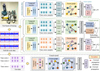 |
Fig. 3 RUL prediction process of the DG-MGNet. |
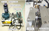 |
Fig. 4 XJTU-SY test bench. |
Cross-domain task configuration.
4.2 Evaluation metrics
We adopt standard evaluation metrics commonly used in PHM studies: root mean squared error (RMSE) and mean absolute error (MAE). Among these, smaller values of RMSE and MAE indicate lower prediction errors and higher accuracy. Furthermore, to better align with the preference for “conservative predictions” in engineering applications, this paper introduces a scoring function to comprehensively evaluate the prediction results. When the model underestimates the RUL, the scoring function applies a higher penalty. The calculation formulas for these metrics and the scoring function are as follows:
 (15)
(15)
 (16)
(16)
 (17)
(17)
where N is the number of test samples, yi denotes the ground-truth value of the i th sample, and  denotes the corresponding predicted value. It should be noted that the RUL label used in this study is a relative remaining-life indicator constructed according to the full degradation sequence of each bearing, rather than an absolute physical quantity. Therefore, the vertical axis in the RUL prediction curves represents the relative RUL value used for model training and evaluation.
4.3 Feature extraction
The quality of feature extraction directly affects the effectiveness of subsequent multi-branch encoding and feature map structure modeling. In this paper, complementary information is extracted from both the time domain and frequency domain perspectives. A total of 14 features are extracted for each directional signal. To avoid instability in training due to differences in units and scales, the features are normalized. Detailed information about all the features is presented in Table 3.
It should be noted that, during the early healthy stage of bearing operation, vibration signals may be relatively stable and contain only weak degradation information. Therefore, the proposed model does not identify early degradation based on a single instantaneous amplitude variation. Instead, it distinguishes early weak degradation from normal operating noise by using temporal continuity and multi-feature consistency. Random operating noise is usually transient and isolated, whereas early degradation tends to cause slight but persistent co-variation among amplitude-energy features, impact-sensitive statistical features, and frequency-domain features. In DG-MGNet, the temporal encoder captures the evolution trend within each feature node, the graph topology models the coupling relationships among different feature channels and sensor directions, and attention pooling emphasizes more informative degradation descriptors.
Definitions of the extracted features.
4.4 Model configuration
This section describes the network architecture and training configuration of the proposed DG-MGNet. The settings of the key modules are summarized in Table 4.
To obtain better predictive performance while keeping the computational cost manageable, cross-validation is employed to select key hyperparameters of DG-MGNet. After determining the optimal configuration, the model is trained on the training set and then used to output RUL predictions on the test set. To reduce variability caused by random initialization and mini-batch sampling, all experiments are repeated 25 times, and the reported results are averaged over these runs. The training hyperparameters are summarized in Table 5.
For the two learning rates in the meta-learning framework, the inner-loop learning rate controls the rapid adaptation of the graph module, while the outer-loop learning rate controls the stable update of the shared initialization. Therefore, the inner-loop learning rate is set larger than the outer-loop learning rate. A relatively larger inner-loop learning rate helps the task graph respond quickly to condition-specific topology changes, whereas a smaller outer-loop learning rate avoids unstable oscillations in the shared parameters during meta-optimization. Based on cross-validation, the inner-loop learning rate and outer-loop learning rate are set to 0.01 and 0.001, respectively.
Detailed structure of DG-MGNet.
The hyperparameters of DG-MGNet.
4.5 Experimental results and analysis
Figure 5 presents the RUL prediction results of several test bearings under six cross-condition transfer tasks, including the ground-truth RUL curves, the predicted curves, the corresponding 95% confidence intervals, and the distribution of prediction errors. It can be observed that, across different condition-transfer scenarios, the proposed DG-MGNet closely follows the true degradation trajectories. The predicted curves exhibit an overall trend consistent with the ground truth, indicating that the model can capture degradation dynamics in a stable manner. From the prediction process, as the bearings gradually enter the late degradation stage, fluctuations or local deviations appear for some cases. For example, in Task 2-Br3_2 and Task 4-Br3_4, the magnitude of prediction errors increases. This suggests that, under severe degradation, bearing conditions are more strongly affected by random shocks and non-stationary noise, and the degradation rate becomes highly nonlinear, which makes accurate prediction more challenging. Notably, although short-term oscillations may occur in the late stage for a few bearings, the model still tracks the overall life-decay path effectively, demonstrating the robustness and generalization capability of the proposed framework.
Table 6 reports the detailed RUL prediction results. Overall, the cross-condition training configuration has a noticeable influence on prediction performance. Under the same target condition, models trained with different source conditions can differ in both accuracy and stability, mainly because the match between source and target conditions varies in terms of load level, rotational speed, and degradation patterns. Nevertheless, even for tasks with large domain gaps, DG-MGNet maintains strong predictive performance, further validating its effectiveness for complex cross-condition bearing RUL prediction.
The accuracy of the RUL predictions in Table 6 is validated based on the known run-to-failure records of the XJTU-SY dataset. Since each tested bearing is operated until failure, the complete degradation sequence length and final failure point are available. For a test bearing with a full-life sequence length Lb, the ground-truth RUL label of the k-th sample is constructed according to its remaining position in the degradation sequence. The model prediction  is then compared with the corresponding ground-truth label yk over the entire test trajectory. RMSE, MAE, and Score are calculated from these point-wise prediction errors, as defined in equations (15)–(17). Therefore, Table 6 provides a quantitative validation of RUL prediction accuracy for each left-out test bearing under the six cross-condition tasks.
To further validate the performance of the proposed method, we conducted a comparative analysis with several state-of-the-art transfer learning methods, including DCDAN [34], TCNN [35], DFDTLN [36], CADA [37], and TACNN [38]. The original data were normalized to facilitate comparative observation. Figure 6 compares the RMSE and MAE achieved by different methods across the six prediction tasks.
As can be seen, the proposed DG-MGNet obtains the lowest or near-lowest RMSE and MAE in all tasks, demonstrating stable and consistent advantages. This indicates that DG-MGNet delivers higher overall prediction accuracy under various cross-condition transfer scenarios. In more challenging settings, DG-MGNet shows particularly strong performance. For Task 2, DG-MGNet achieves an RMSE of 0.1528, which is 2.9% lower than DCDAN and 12.9% lower than CADA. For Task 4, DG-MGNet attains an RMSE of 0.1531, outperforming TCNN by 13.5% and DFDTLN by 15.2%, highlighting its stronger robustness when the domain gap between operating conditions is large. In addition, CADA exhibits relatively large error fluctuations across several tasks, suggesting limited stability in cross-domain prediction. Notably, DG-MGNet shows highly consistent trends on RMSE and MAE, with smaller cross-task variations, implying a more stable overall distribution of prediction errors. The improved performance of DG-MGNet can be mainly attributed to two aspects: (i) the multi-level dynamic graphs capture richer structural dependencies, and (ii) the meta-learning mechanism enables the task-graph topology to adapt to changing operating conditions, enhancing generalization and allowing the model to maintain reliable prediction performance under cross-condition transfer.
It should also be noted that the experimental signals in the XJTU-SY dataset are real vibration measurements, and therefore inevitably contain measurement noise caused by sensor acquisition, installation conditions, and environmental disturbances. In the proposed DG-MGNet, the influence of ordinary measurement noise is reduced mainly through multi-feature representation, temporal encoding, graph-based coupling modeling, and attention pooling. Random measurement noise is usually transient and weakly correlated across multiple feature channels, whereas bearing degradation tends to produce more persistent and coupled changes among time-domain energy features, impact-sensitive statistical features, and frequency-domain features. Therefore, the model can suppress isolated fluctuations to some extent and focus on degradation-related consistent patterns. However, under extremely strong noise conditions, degradation information may be severely masked, and the prediction accuracy may decrease. In such cases, additional denoising preprocessing or noise-adaptive training would be required, which will be further investigated in future work.
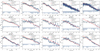 |
Fig. 5 RUL prediction curves for partial bearings. |
Detailed results of RUL prediction.
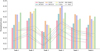 |
Fig. 6 Comparison results of different models. |
4.6 Computational efficiency analysis
To further evaluate the engineering practicality of DG-MGNet, we compare the computational efficiency of different models under the same hardware and software configurations. Table 7 reports the average training time per epoch and inference time per sample.
As shown in Table 7, DG-MGNet requires 132.7 ms per training epoch and 2.36 ms per test sample. Although the proposed model introduces multi-level graph construction, task-adaptive graph generation, and meta-learning optimization, its computational overhead remains moderate. Compared with the fastest baseline, CADA, DG-MGNet increases the training time by 17.6%, but it is still more efficient than DCDAN, DFDTLN, and TACNN. Moreover, the inference time remains at the millisecond level because the inner–outer loop optimization is only used during training. Therefore, DG-MGNet achieves improved prediction performance with acceptable computational cost and is feasible for periodic online RUL updating in practical condition-monitoring systems.
Comparison of computational efficiency for different models.
5 Discussion
This section investigates the key mechanisms and performance drivers of DG-MGNet, focusing on ablation studies, adjacency-matrix visualization, and feature-space visualization before and after graph modeling. These analyses provide further insight into the internal workings of the proposed method and its role in cross-condition RUL prediction.
5.1 Ablation study
To further quantify the contribution of each key component in DG-MGNet and to identify the sources of performance improvements, we conduct ablation experiments under the same six cross-condition task splits and data preprocessing settings as in the comparative experiments. Except for the removed or replaced module, the remaining network architecture, training strategy, and hyperparameter settings are kept unchanged. Figure 7 reports the normalized RMSE and MAE of different ablation variants across the six tasks. Overall, the full model achieves the lowest error in all tasks, indicating that multi-level graph-structure modeling and the meta-learning optimization strategy jointly enhance the stability and accuracy of cross-condition RUL prediction.
When the meta-learning adaptation mechanism is removed, prediction errors increase consistently, with the average RMSE rising to 0.1580 and the average MAE to 0.1288. The degradation is more pronounced in tasks with larger transfer difficulty: in Task 2, RMSE increases by 0.0190, and in Task 4 by 0.0229. These results suggest that parameters learned via standard static training are insufficient to accommodate distribution changes in the target condition, whereas the inner-outer loop updates in meta-learning facilitate task-level adjustment and thus reduce performance loss during cross-domain transfer. This result further verifies the effectiveness of the meta-learning mechanism. Since only the inner–outer loop adaptation is removed, the increased errors of the w/o Meta variant indicate that static graph parameters are insufficient to capture task-specific topology drift, while the proposed meta-learning strategy improves rapid cross-condition generalization. Removing the task-adaptive graph also leads to a clear performance drop, with the average RMSE increasing to 0.1535. This indicates that, under cross-condition settings, the coupling relationships among monitoring variables are not fixed, and relying solely on shared structures is insufficient to capture task-specific relational changes. Moreover, eliminating the multi-level fusion structure results in a 15% increase in the average RMSE, implying that the fused design better balances shared stability and task adaptivity. In addition, replacing attention pooling with simple mean pooling increases the average RMSE to 0.1501; in particular, the RMSE of Task 4 rises from 0.1531 to 0.1638. This demonstrates that different nodes contribute unequally to degradation representation, and attention aggregation can emphasize nodes that are more informative for the degradation process, yielding more robust graph-level embeddings.
In summary, the effectiveness of DG-MGNet stems from two complementary aspects. Multi-level modeling of structural dependencies provides a stable and transferable topological prior, while meta-learning-driven rapid adaptation of task topology further strengthens the model’s generalization capability under varying operating conditions.
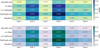 |
Fig. 7 Results of ablation experiment. |
5.2 Adjacency matrix visualization
To further uncover the structural reasons behind the performance gains of DG-MGNet in cross-condition RUL prediction, and to verify whether the proposed method can learn interpretable feature dependency patterns, we visualize the adjacency matrices generated by the model. By comparing the multi-level fused adjacency matrix with the adaptively generated task-specific adjacency matrix, we examine how the model captures correlations under different sources of structural constraints.
The visualization results for cross-condition tasks are shown in Figure 8. It can be observed that the fused adjacency matrix exhibits relatively high and evenly distributed weights along the main diagonal. This suggests that, during information propagation, the model prioritizes preserving each node’s own degradation representation and uses it as a stable basis for cross-node interactions. Such a structure helps prevent feature mixing caused by overly strong inter-node coupling, and indicates that the multi-level fusion mechanism provides balancing and regularization across different structural sources, leading to a more stable graph topology. From a physical perspective, this diagonal-dominant pattern is consistent with the fact that each vibration feature first carries its own degradation information, while the off-diagonal connections further describe correlated changes among time-domain impact features, energy-related features, and frequency-domain features.
In contrast, the task-specific adjacency matrix is noticeably sparser, with several prominent vertical high-weight bands and locally enhanced regions. This indicates that, for the current task, a small number of key nodes maintain strong connections with many other nodes. These nodes act as hubs during graph propagation, enabling condition-relevant global degradation information to be aggregated and more effectively transmitted to other nodes. These observations demonstrate that the task graph can dynamically adjust inter-node coupling according to target-domain samples, thereby characterizing changes in correlation structures under different operating conditions. This sparse topology also suggests that, under different speed-load combinations, only a limited number of feature channels may dominate the degradation representation, which is consistent with the condition-dependent nature of bearing fault propagation and vibration response.
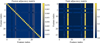 |
Fig. 8 Visualization of adjacency matrices. |
5.3 Feature space visualization
To examine the degradation consistency of learned representations under cross-condition settings, we apply t-SNE to visualize features before and after graph-structure modeling. Figure 9 presents three sets of visualization results. The color of each point indicates the normalized life level, where the color gradually changes from dark to light as degradation evolves from an early stage toward failure.
As shown in Figure 9, when structural dependencies are not sufficiently modeled, the feature distribution tends to appear as scattered clusters, and the colors are interleaved in the embedding space. This indicates that samples from different life stages cannot form a stable and continuous transition in the feature space. In contrast, after graph modeling, the features exhibit a much clearer low-dimensional manifold: points are smoothly distributed along a continuous trajectory, and the color gradient evolves monotonically along the direction of this trajectory. In other words, life stages can be organized in the feature space as a continuous path from healthy to degraded conditions. Such a geometric structure suggests that the learned representations better align with the intrinsic evolution of the degradation process. On the one hand, samples from different life stages present a more stable ordering relationship in the embedding space, improving the interpretability of the representation with respect to degradation progression. On the other hand, the transition from scattered clusters to a continuous trajectory implies stronger degradation-semantic alignment across operating conditions, reducing the interference of condition discrepancies on the representation space.
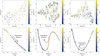 |
Fig. 9 Visualization of the features: (a) bearing1_2, (b) bearing2_3, (c) bearing3_3. |
6 Conclusion and future work
6.1 Conclusion
This paper addresses the distribution shift and unstable generalization issues in cross-condition bearing RUL prediction. We propose DG-MGNet and validate it on a public accelerated bearing life dataset. The main work and conclusions are summarized as follows.
We propose a graph-aware meta-learning framework for domain generalization. To tackle the performance degradation caused by changes in the statistical properties of monitoring signals under different operating conditions, we extend bearing degradation modeling from sequence learning to structured representation learning, and jointly leverage graph modeling and meta-learning to enhance cross-condition prediction. At the task level, the framework alleviates distribution shift induced by operating-condition variations through dynamic adaptation, and improves stability across different transfer tasks.
We construct multi-level dynamic adjacency relationships to capture degradation-related dependencies. By integrating prior structure, globally shared structure, and task-adaptive structure, we build a multi-level dynamic adjacency matrix. This design enables the graph topology to remain stable while being adaptive, thereby improving the transferability of cross-condition degradation representations from a structural perspective.
We design a meta-learning-driven strategy for rapid task-topology updates. During training, an inner–outer loop joint optimization scheme is introduced to adapt graph-generation-related parameters at the task level, enabling task-specific topology to quickly adjust as operating conditions change and thus reducing performance loss caused by cross-domain transfer. Experimental results show that this strategy effectively mitigates results show that this strategy effectively mitigates performance degradation in more challenging transfer tasks, demonstrating stronger robustness and generalization.
In summary, DG-MGNet provides an effective domain-generalization solution for bearing RUL prediction under complex operating conditions, offering methodological support for predictive maintenance and O&M decision optimization.
6.2 Future work
Future work will focus on more realistic cross-condition RUL prediction scenarios involving multi-source sensing data, and on deployment-oriented model designs that reduce computational cost while supporting efficient online adaptation and maintenance decision-making.
Acknowledgments
The authors would like to thank their institutions and colleagues for their administrative and technical support in this work.
Funding
The research was supported by the Guangxi Key Research and Development Program (No. Guike AB23026120), the Major Science and Technology Special Project of Nanning (No. 20231029), the Guangxi Natural Science Foundation Youth Fund Project (No. 2025JJB160249), and the Yongjiang Program for Young Talents (No. RC20240104).
Conflicts of interest
C. Zexian Wei has received funding from the Guangxi Key Research and Development Program (No. Guike AB23026120), the Major Science and Technology Special Project of Nanning (No. 20231029), the Guangxi Natural Science Foundation Youth Fund Project (No. 2025JJB160249), and the Yongjiang Program for Young Talents (No. RC20240104). A. Zhaohui Wu, B. Qiang Chen, D. Yehua Ling, E. Guoxi Hou, F. Yong Zhou, and G. Yong Zhou certify that they have no financial conflicts of interest in connection with this article.
Data availability statement
The data supporting the findings of this study are available from the corresponding author upon reasonable request.
Author contribution statement
Conceptualization, Zhaohui Wu and Zexian Wei; Methodology, Zhaohui Wu and Zexian Wei; Validation, Zhaohui Wu, Qiang Chen, Yehua Ling and Guoxi Hou; Investigation, Zhaohui Wu, Qiang Chen, Pinjie Zhao and Guoxi Hou; Data Curation, Zhaohui Wu and Qiang Chen; Writing – Original Draft Preparation, Zhaohui Wu; Writing – Review & Editing, Zexian Wei, Pinjie Zhao and Yong Zhou; Visualization, Zhaohui Wu; Supervision, Zexian Wei, Yehua Ling and Yong Zhou; Project Administration, Zexian Wei; Funding Acquisition, Zexian Wei.
References
- I. Sabahi, M. Vermaut, M. Kirchner, Z. Li, K. Gryllias, F. Naets, Bearing housing as a sensor: estimation of lumped bearing loads using accurate housing models, Mech. Syst. Signal Process. 242, 113591 (2026) [Google Scholar]
- J. Koutsoupakis, D. Giagopoulos, A simulation-enhanced deep learning framework for bearing fault diagnosis using an improved bearing force model, Mech. Syst. Signal Process. 241, 113519 (2025) [Google Scholar]
- C. Deng, J. Lu, L. An, Z. Gao, X. Cheng, C. Tian, A friction temperature model for dynamic operating bearing based on CNN and CNNLSTM, Eng. Appl. Artif. Intell. 160, 112042 (2025) [Google Scholar]
- D. He, J. Zhao, Z. Jin, C. Huang, F. Zhang, J. Wu, Prediction of bearing remaining useful life based on a two-stage updated digital twin, Adv. Eng. Inform. 65, 103123 (2025) [Google Scholar]
- X. Ma, Z. Li, J. Xiang, X. Sun, C. Chen, F. Huang, Nonlinear vibration analysis of rotor-bearing system with insufficient interference and bearing tilt, Int. J. Mech. Sci. 287, 109966 (2025) [Google Scholar]
- R. Zhang, C. Song, Y. Zhou, J. Tan, Z. Zeng, Tribodynamic behavior of a novel double bearing layout for the main shaft system of wind turbines, Tribol. Int. 204, 110496 (2025) [Google Scholar]
- L. Wang, X. Ding, X. Liu, J. Cai, R. Li, Optimization and multiphysics coupling analysis of high bearing capacity for wind turbine gearbox sliding bearings, Tribol. Int. 214, 111162 (2026) [Google Scholar]
- Q. Zhao, X. Zhang, J. Xie, S. Liang, E. Mbeka, KFC-Former: an interpretable kernel function convolutional-former with phase space reconstruction for remaining useful life prediction of mechanical equipment, Expert Syst. Appl. 302, 130472 (2026) [Google Scholar]
- Q. Li, X. Xiong, J. Ren, Remaining useful life prediction based on degradation-aware dynamic graph representation learning, Eng. Appl. Artif. Intell. 163, 113140 (2026) [Google Scholar]
- Y. Yuan, Y. Han, K. Xiao, Z. Xu, X. Jiang, Remaining useful life prediction for the harmonic reducer of industrial robots via in-situ current signal and lightweight multiscale attention deep networks, J. Manuf. Syst. 83, 322–336 (2025) [Google Scholar]
- T. Xia, X. Xing, T. Yan, D. Wang, E. Pan, L. Xi, Interpretable temporal degradation state chain based fusion graph for intelligent bearing fault detection, Adv. Eng. Inform. 59, 102342 (2024) [Google Scholar]
- A. Cao, H. Gao, S. Fan, L. Guo, Z. You, Y. Lei, Y. Sun, J. He, Study on vibration mechanism and dynamic characteristics for TBM main bearing defects, Mech. Syst. Signal Process. 222, 111807 (2025) [Google Scholar]
- Z. Yin, F. Zhang, C. Yin, G. Xu, S. Liu, A bearing fault diagnosis method for sample imbalance, Eng. Appl. Artif. Intell. 157, 111171 (2025) [Google Scholar]
- S. Wu, P. Shi, X. Xu, X. Yang, R. Li, Z. Qiao, KMDSAN: a novel method for cross-domain and unsupervised bearing fault diagnosis, Knowl.-Based Syst. 312, 113170 (2025) [Google Scholar]
- D. He, J. Zhao, Z. Jin, C. Huang, C. Yi, J. Wu, DCAGGCN: a novel method for remaining useful life prediction of bearings, Reliab. Eng. Syst. Saf. 260, 110978 (2025) [Google Scholar]
- Y. Du, X. Geng, Q. Zhou, S. Cheng, H. Zhang, Dynamic preventive maintenance model for offshore wind turbine bearings based on remaining useful life prediction, Sustain. Energy Technol. Assess. 84, 104750 (2025) [Google Scholar]
- R. Guo, J. Yi, X. Luo, An efficient classification and error correction knowledge distillation framework for remaining useful life prediction of bearings in air turbine starter, Neurocomputing 657, 131611 (2025) [Google Scholar]
- G. Li, J. Wei, J. He, H. Yang, F. Meng, Implicit Kalman filtering method for remaining useful life prediction of rolling bearing with adaptive detection of degradation stage transition point, Reliab. Eng. Syst. Saf. 235, 109269 (2023) [Google Scholar]
- X. Si, H. Li, Z. Zhang, N. Li, A Wiener-process-inspired semi-stochastic filtering approach for prognostics, Reliab. Eng. Syst. Saf. 249, 110200 (2024) [Google Scholar]
- Y. Jin, D. Liu, Y. Xiao, L. Cui, Dual-channel dynamic spline graph convolutional network for bearing remaining useful life prediction, Reliab. Eng. Syst. Saf. 266, 111731 (2026) [Google Scholar]
- W. Yin, H. Xia, E. Zio, X. Huang, Deep ensemble learning and error correction method for remaining useful life prediction of rolling bearings, Eng. Appl. Artif. Intell. 161, 112128 (2025) [Google Scholar]
- Z. Pan, X. Pan, F. Jiang, Y. Wu, Z. Meng, Y. Wang, P. Zhao, W. Lu, Remaining useful life prediction of rolling-element bearings based on cumulative transformation and EResNet-KSLSTM network, Mech. Syst. Signal Process. 238, 113251 (2025) [Google Scholar]
- M. Furqon, M. Pratama, L. Liu, H. Habibullah, K. Dogancay, Mixup domain adaptations for dynamic remaining useful life predictions, Knowl.-Based Syst. 295, 111783 (2024) [Google Scholar]
- J. Shang, D. Xu, X. Shang, C. Zhao, C. Jiang, H. Qiu, L. Gao, CITDG: a causality and information-theory inspired domain generalization method for machine remaining useful life prediction in unseen domains, Mech. Syst. Signal Process. 241, 113527 (2025) [Google Scholar]
- J. Du, L. Song, X. Gui, J. Zhang, L. Guo, X. Li, Remaining useful life prediction under variable operating conditions via multisource adversarial domain adaptation networks, Appl. Soft Comput. 161, 111717 (2024) [Google Scholar]
- C. Wu, C. Ma, J. He, C. Fang, L. Wang, X. Jin, Y. Liu, Consider the sample-weighted multi-source partial domain adaptation network for remaining useful life prediction under incomplete target data, Adv. Eng. Inform. 68, 103775 (2025) [Google Scholar]
- H. Tian, J. Mi, S. Tong, Y.-F. Li, Uncertainty-weighted with gradient-based to re-weight domain generalization for remaining useful life prediction of rotating machinery under unseen conditions, Reliab. Eng. Syst. Saf. 267, 111810 (2026) [Google Scholar]
- W. Mao, R. Guo, J. Wang, M. Zuo, Z. Zhong, Wiener process-assisted online remaining useful life prediction with deep incremental regression transfer learning, Reliab. Eng. Syst. Saf. 267, 111867 (2026) [Google Scholar]
- T. Liu, Y. Li, Z. Hu, C. Fu, G. Song, Remaining useful life prediction of bearings based on small-sample enhanced and interpretable transfer learning, Adv. Eng. Inform. 69, 103938 (2026) [Google Scholar]
- Z. Men, D. Gong, K. Zhou et al., Unsupervised domain adaptation method for bearing fault diagnosis assisted by twin data under extreme sample scarcity, Mech. Syst. Signal Process. 239, 113359 (2025) [Google Scholar]
- Z. Men, Y. Li, L. Gao et al., Fault diagnosis method for railway wagon bearings under imbalanced dataset based on improved ACWGAN, Nonlinear Dyn. 113, 14935–14962 (2025) [Google Scholar]
- J. Zhao, D. He, Z. Jin, X. Zhang, J. Zhou, A new method for bearing remaining useful life prediction based on dynamic wavelet and physical information constraints, Expert Syst. Appl. 296, 129023 (2026) [Google Scholar]
- B. Wang, Y. Lei, N. Li, N. Li, A hybrid prognostics approach for estimating remaining useful life of rolling element bearings, IEEE Trans. Reliab. 69, 401–412 (2020) [Google Scholar]
- Y. Zhang, X. Zhao, Z. Peng, R. Xu, Y. Hui, Cross-domain remaining useful life prediction for rolling bearings based on wavelet decomposition and dynamic calibrated domain adaptive networks, Measurement 251, 117278 (2025) [Google Scholar]
- H. Cheng, X. Kong, G. Chen, Q. Wang, R. Wang, Transferable convolutional neural network based remaining useful life prediction of bearing under multiple failure behaviors, Measurement 168, 108286 (2021) [Google Scholar]
- T. Hu, Y. Guo, L. Gu, Y. Zhou, Z. Zhang, Z. Zhou, Remaining useful life prediction of bearings under different working conditions using a deep feature disentanglement based transfer learning method, Reliab. Eng. Syst. Saf. 219, 108265 (2022) [Google Scholar]
- M. Ragab, Z. Chen, M. Wu, C.S. Foo, C.K. Kwoh, R. Yan, X. Li, Contrastive adversarial domain adaptation for machine remaining useful life prediction, IEEE Trans. Ind. Inform. 17, 5239–5249 (2021) [Google Scholar]
- S. Xie, W. Cheng, Z. Nie, J. Xing, X. Chen, L. Gao, Z. Xu, R. Zhang, Multidimensional attention domain adaptive method incorporating degradation prior for machine remaining useful life prediction, IEEE Trans. Ind. Inform. 20, 7345–7356 (2024) [Google Scholar]
Cite this article as: Zhaohui Wu, Qiang Chen, Zexian Wei, Yehua Ling, Guoxi Hou, Pinjie Zhao, Yong Zhou, A graph-aware meta network for domain generalization in cross-condition bearing RUL prediction, Int. J. Metrol. Qual. Eng. 17, 11 (2026), https://doi.org/10.1051/ijmqe/2026009
All Tables
All Figures
|
Fig. 1 Different types of monitoring data. |
| In the text | |
|
Fig. 2 Degradation feature extraction based on multi-scale graph. |
| In the text | |
|
Fig. 3 RUL prediction process of the DG-MGNet. |
| In the text | |
|
Fig. 4 XJTU-SY test bench. |
| In the text | |
|
Fig. 5 RUL prediction curves for partial bearings. |
| In the text | |
|
Fig. 6 Comparison results of different models. |
| In the text | |
|
Fig. 7 Results of ablation experiment. |
| In the text | |
|
Fig. 8 Visualization of adjacency matrices. |
| In the text | |
|
Fig. 9 Visualization of the features: (a) bearing1_2, (b) bearing2_3, (c) bearing3_3. |
| In the text | |
Current usage metrics show cumulative count of Article Views (full-text article views including HTML views, PDF and ePub downloads, according to the available data) and Abstracts Views on Vision4Press platform.
Data correspond to usage on the plateform after 2015. The current usage metrics is available 48-96 hours after online publication and is updated daily on week days.
Initial download of the metrics may take a while.