


| Issue |
Int. J. Metrol. Qual. Eng.
Volume 17, 2026
|
|
|---|---|---|
| Article Number | 16 | |
| Number of page(s) | 13 | |
| DOI | https://doi.org/10.1051/ijmqe/2026012 | |
| Published online | 22 July 2026 | |
Research Article
Fault detection and diagnosis of electric vehicle battery pack combining neural network and CRDAN algorithm
Intelligent Manufacturing School, Nanchong Vocational College of Science and Technology, Nanchong 637200, PR China
* Corresponding author: This email address is being protected from spambots. You need JavaScript enabled to view it.
Received:
22
September
2025
Accepted:
8
June
2026
Abstract
With the widespread use of electric vehicles, higher standards for battery pack safety and reliability have emerged, making fault detection and diagnosis essential for stable operation. This study proposes a two-stage approach that combines a convolutional neural network (CNN) and bidirectional long short-term memory (BiLSTM) for fault detection, followed by a fault diagnosis model integrating a domain-adaptive neural network with channel attention, temporal attention, and category enhancement mechanisms. The detection model achieved maximum accuracy of 97.53%, precision of 98.03%, F1 score of 0.998, and recall of 99.31%, with minimum RMSE of 0.004 and time consumption of 49 ms, significantly outperforming comparison models. For diagnosis, the model achieved an AUC of 0.987, diagnostic accuracy of 98.33%, and time consumption of 66 ms, while demonstrating higher precision in identifying short-circuit, over-charging, over-discharging, and capacity fading faults. The proposed detection and diagnostic framework operates with high efficiency and robustness, offering reliable technical support for the safe operation and maintenance of electric vehicle battery packs.
Key words: CNN / BiLSTM / fault / detection / diagnosis / electric vehicle / lithium battery
© L. Wu, Published by EDP Sciences, 2026
 This is an Open Access article distributed under the terms of the Creative Commons Attribution License (https://creativecommons.org/licenses/by/4.0), which permits unrestricted use, distribution, and reproduction in any medium, provided the original work is properly cited.
1 Introduction
Electric vehicles (EVs), a kind of clean energy transportation, are steadily emerging as a key area of future development in the transportation sector due to their many benefits, including high efficiency and environmental protection [1,2]. However, the battery pack (BP), which is one of the core components of EVs, may suffer from various failures, such as short circuits and battery cell capacity fade, during long-term operation [3]. These malfunctions may result in safety incidents in addition to impairing the vehicle's ability to operate normally. Therefore, to guarantee the security and dependability of the cars, efficient fault detection (FDE) and diagnosis of BPs in EVs is essential. To address this problem, some of the commonly used methods are convolutional neural network (CNN), bidirectional long short term memory (BiLSTM), support vector machine (SVM), equivalent circuit modeling method, D-S evidence theory fusion methods, etc [4,5]. Meanwhile, more and more scholars have launched research on this problem.
Sepasiahooyi S et al. designed a model based detection method in order to perform FDE for battery management system of EVs. Two adaptive observers were used in the method's design to identify issues with the voltage sensor and the condition of charge, respectively. The outcomes revealed that the designed observers could accurately detect the faults of seven years old and new batteries [6]. Shen J W et al. designed a method based on data mining and extensive data analysis in an effort to perform fault diagnosis (FDI) and anomaly detection for EV batteries. The method visualized the dimensionality reduction of the electric cell data by t-distributed stochastic neighborhood embedding algorithm. The results indicated that the method had good FDI and anomaly detection performance [7]. Kim W et al. developed a nonlinear model-based technique that uses normalized residuals, a state observer, and a disturbance observer to identify current sensor issues in EV battery management systems. The method's good detection performance at various current intensities was demonstrated by the results [8]. Xia M N et al. built fault models of a few common circuits and a model of the charging and discharging (CD) process of EV power batteries in an attempt to diagnose charging issues in EVs. To diagnose the gathered fault data, an enhanced whale algorithm was also created. The results indicated that the method had a high diagnostic accuracy and a fast diagnostic speed [9].
The current methods for detecting and diagnosing battery faults in electric vehicles are mainly divided into four categories: (1) Model driven methods, which rely on equivalent circuit models and state observers to achieve fault diagnosis, rely on accurate battery modeling, and have poor adaptability under complex working conditions; (2) Traditional machine learning methods, such as SVM, random forest, and extreme learning machines, rely on manual design for feature extraction and have limited ability to handle high-dimensional temporal data; (3) A single deep learning method, one-dimensional (1D) CNN excels in local features but lacks temporal modeling, while BiLSTM excels in temporal dependencies but lacks local feature extraction; (4) Domain adaptation and attention methods often lack category enhancement mechanisms, which limits the accuracy of fault classification. The above methods are difficult to simultaneously meet the high-precision, strong temporal, and high generalization requirements of battery fault detection. Therefore, to detect and diagnose the faults of EV BPs, the study combines the respective advantages of 1D CNN and BiLSTM to construct a FDE model. It also proposes a FDI model using category revitalization mechanism-attention module (AM)-domain adaptation neural network (CRDAN). In addition to offering fresh concepts and approaches for the creation of next EV FDE and FDI procedures, the research seeks to offer robust technical support for the safe operation and maintenance of EV BPs.
The innovation of this paper lies in: (1) Building a one-dimensional CNN BiLSTM fusion fault detection model, combining the advantages of CNN local feature extraction and BiLSTM timing dependency capture capability, to solve the problem of incomplete feature extraction of a single model. (2) Propose a CRDAN diagnostic algorithm that integrates channel attention, time attention, and category enhancement mechanisms. By using domain adaptation to reduce the impact of operating condition differences, dual attention is used to enhance key features, and category enhancement is used to improve the accuracy of fault type discrimination. The algorithm architecture achieves full chain optimization of feature extraction domain adaptation fault classification.
2 Methods and materials
The article develops an FDE approach based on a 1D CNN-BiLSTM neural network and builds an FDI model taking into account FDE and CRDAN in order to identify and diagnose the flaws of EV BPs. Furthermore, this FDI model involves the channel AM and the time AM.
2.1 Design of FDE method considering neural network CNN and BiLSTM
To detect and diagnose the faults of EV BPs, the study firstly designs a FDE method combining 1D CNN and BiLSTM neural networks, and uses its detection data as the input for the subsequent FDI model. Second, the study designs a CRDAN diagnosis model. EV BPs are mainly lithium-ion (LI) batteries, and the CD process of power lithium battery (PLE) is a complex physicochemical process. The process is schematically shown in Figure 1 [10,11].
In Figure 1, the migration of LIs between the positive and negative electrodes is a component of the CD process of the PLE, and the cathode, anode, and electrolyte are the fundamental components of the LI battery. In addition, when the PLE is CD, its internal structures such as electrode materials and electrolyte undergo various chemical reactions, which directly affect the performance and lifetime of the battery. For instance, the lattice structure of the cathode material may undergo expansion or contraction due to the embedding/de-embedding of LIs, and the solvent molecules in the electrolyte may react with the electrode material in a side reaction. Moreover, the battery's lifespan and performance will be affected by all of these modifications. Therefore, by monitoring the changes of voltage, current, temperature and other parameters in the CD process, the abnormal state of the battery can be detected in time, which provides an important basis for FDE. Since most of the battery parameter data are one-dimensional, the study employs a 1D CNN for feature extraction.
One deep learning model that is specifically designed to process one-dimensional data is called 1D CNN. With the benefits of local feature extraction, parameter sharing, translation invariance, reduced computation, and scalability, it processes sequence data effectively. Its uses are more extensive in the domains of time series analysis, signal processing, and FDE. The structure of 1D CNN mainly contains an input layer, a convolutional layer, an activation function (AF), a pooling layer, a fully connected layer (FCL), and an output layer (OL). Among them, the output ai expression of the convolutional layer is shown in equation (1) [12].
 (1)
(1)
In equation (1), i represents the index of the output feature. B(∙) is the AF. ci is the weight matrix (WM). di is the input. fi is the bias vector. * is dot product operation. For the AF, the study uses scaled exponential linear unit (SELU). SELU is a kind of self-normalized AF, which can not only speed up the convergence of the neural network, but also mitigate overfitting. The specific expression of SELU is shown in equation (2) [13].
 (2)
(2)
In equation (2), g represents the scaling parameter. h represents the control parameter. Meanwhile, the values of g and h are usually 1.0507 and 1.6732. Equation (3) displays the formula for the maximum pooling operation.
 (3)
(3)
In equation (3),  represents the result of the pooling operation. ki and ki−1 are two neighboring eigenvalues, respectively. The solution of the pooled eigenvalue li is shown in equation (4).
 (4)
(4)
In equation (4), mi is the deviation. Therefore, the final output vector ni is expressed as shown in equation (5).
 (5)
(5)
In equation (5), pi represents the deviation. oi is the WM. In addition, the input of one-dimensional CNN is normalized time-series data of battery voltage, current, temperature, and capacity, and the output is a local abstract feature vector. During training, the one-dimensional CNN uses the Adam optimizer with a learning rate of 0.001 and backpropagation to update the convolution kernel and bias. After feature extraction by 1D CNN, the study uses BiLSTM neural network to obtain the correlation between the data. BiLSTM neural network is a special kind of recurrent neural network. It is able to process sequential data and maintain long-term memory, and is better able to capture contextual relationships in sequential data. The advantages of BiLSTM include enhanced contextual understanding, improved accuracy and versatility. Time series analysis, FDE, and natural language processing are just a few of its many uses [14]. The structure of BiLSTM mainly consists of two LSTM layers, i.e., a forward LSTM and an inverse LSTM. Moreover, each LSTM cell contains input gates (IGs), forgetting gates (FGs), output gates (OGs) and cell states. Among them, the FG expression rt of the forward LSTM is displayed in equation (6) [15].
 (6)
(6)
In equation (6), s represents the Sigmoid AF with output range (0, 1). wr represents the WM of the FG. ut−1 is the hidden state (HS) of t−1 at the previous moment. vt represents the input of t at the current moment. br represents the bias term (BT) of the oblivious gate. The IG expression yt of the forward LSTM is shown in equation (7).
 (7)
(7)
In equation (7), wy represents the WM of the IG. by is the BG of the IG. The OG expression zt of the forward LSTM is shown in equation (8).
 (8)
(8)
In equation (8), wz and bz represent the WM and BG of the OG, respectively. The formula for the reverse LSTM is similar to the forward LSTM, but the input sequence is reversed. That is, it is computed forward from the last time step. Therefore, the HS  expression of BiLSTM is shown in equation (9).
 (9)
(9)
In equation (9),  is the HS of forward LSTM at t.
  represents the HS of the reverse LSTM at t. The final output Dt expression of BiLSTM is shown in equation (10).
 (10)
(10)
In equation (10), wD and bD represent the WM and BG of the FCL. The input of the BiLSTM module is the local features output by one-dimensional CNN, and its output is the global features fused with bidirectional temporal information. And during training, the BiLSTM module and one-dimensional CNN are jointly trained end-to-end, synchronously updating weights and biases. Therefore, the structure of the battery FDE model based on 1D CNN-BiLSTM is shown in Figure 2.
In Figure 2, the battery FDE model mainly contains inputs of discharge time, charging current, capacity parameters, data normalization, 1D CNN, BiLSTM, Dropout layer, FCL, inverse normalization, and battery health status output. Among them, data normalization needs to ensure that the input data is on the same scale. 1D CNN captures local patterns and structural information in the input data, such as the shape of the discharge curve, the characteristics of the charge curve, etc., through convolution operation and pooling operation. BiLSTM recognizes time-series patterns in battery data through two LSTM networks. The Dropout layer needs to randomly discard a portion of neurons to prevent model overfitting. The FCL needs to map the output of the hidden layer to the OL, while the inverse normalization layer needs to reduce the output of the FCL to the original scale and output the battery health status through the OL. Figure 3 depicts the battery FDE model's training and detection flow.
In Figure 3, the battery FDE model training and detection process focuses on solving the 1D CNN layer, BiLSTM layer, OL, and error by combining the training data. Furthermore, when the model does not reach the maximum iteration, the error needs to be solved by backpropagation and used to update the weights and bias. Finally, data inverse normalization is required before outputting the test set detection results.
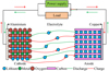 |
Fig. 1 Charging and discharging process of power lithium battery. |
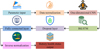 |
Fig. 2 The structure of battery FDE model based on 1D CNN-BiLSTM. |
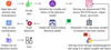 |
Fig. 3 The training and detection process of the battery FDE model. |
2.2 Design of FDI method considering FDE and CRDAN algorithm
The study designed a 1D CNN-BiLSTM based battery FDE model and used its detection data as an input to the FDI model to further analyze the type of fault. For the construction of the FDI model, the study has used domain adaptation neural network, channel AM, temporal AM, and category enhancement mechanism to form the CRDAN algorithm. The structure of the CRDAN module is gradient inversion layer → domain classifier → fault classifier, and it embeds channel attention, time attention, and category enhancement mechanisms. And its input is the fault feature data output by the fault detection model, and its output is the fault domain discrimination result and four types of fault labels: short circuit, overcharge, overdischarge, and capacity attenuation. During training, the CRDAN module utilized minimizing fault classification loss and maximizing domain discrimination loss, with 200 iterations. Domain-adaptive neural network is an artificial neural network architecture and training method for solving cross-domain problems, which has the advantages of reducing the cost of data acquisition and high adaptability [16]. The diagnostic effect of the model will be impacted by variations in the signal properties of lithium batteries under various environmental situations. Therefore, the study utilizes domain-adaptive neural networks to help the FDI model adapt to the differences between different devices, different operating conditions or different fault types, with a view to improving the accuracy and reliability of FDI. The domain adaptation neural network mainly reduces the feature differences by maximizing the loss function of a domain classifier. Moreover, this process will use the Softmax function as shown in equation (11) [17].
 (11)
(11)
In equation (11),  denotes the result of the Gth element of the vector F after the Softmax function. H is the total number of real vectors. The study presents a category augmentation approach to improve the model's recognition of various defect types. The mechanism works by fusing the fault category features J and fault domain features KM. It reinforces the relative importance of the model to the generic fault features, thus enabling the model to recognize and diagnose different types of faults more accurately. The output
  of this mechanism is displayed in equation (12).
 (12)
(12)
In equation (12), IL represents the function. ML represents the feature vector after processing by the multilayer perceptron. ML is the WM. The category enhancement mechanism consists of a fault category feature branch, a fault domain feature branch, a feature fusion layer, and a nonlinear mapping layer. Its input is the domain features output by the domain classifier in the CRDAN network and the category features output by the fault classifier. The output is an enhanced fault discrimination feature that combines category information and domain information, and it is input to the final fault classification layer. In addition, the training method for category enhancement mechanism requires embedding domain adaptive training process to minimize domain distribution differences while maximizing inter category discrimination. The study also adopted joint supervision of category loss and domain loss, and the training process had a fixed iteration of 200 rounds. The channel AM is an attention mechanism which is capable of assigning different weights. Moreover, it emphasizes the features of important channels and has the advantages of computationally efficient, retaining the information integrity of the original channel features and flexibility [18]. Therefore, it is investigated to weight the features of different channels through this module, so as to enhance the features that are useful for FDI and suppress the irrelevant or unimportant features. Figure 4 depicts the channel AM's construction.
In Figure 4, the structure of channel AM contains input feature image, maximum pooling, average pooling, shared FCL, sum by element operation, Sigmoid operation, and channel attention. In addition, the input of the channel attention module is the multi-dimensional temporal feature map output by the fault feature extraction network, and the output is the channel attention weight map with the same dimension as the input feature, which is used to weight the original features in the channel dimension. In addition, the training method of this module is end-to-end joint training with the CRDAN diagnostic network, with fault classification loss and domain adaptive loss as optimization objectives, and updating the shared fully connected layer weights and biases through backpropagation. The expression of channel attention IN is shown in equation (13).
 (13)
(13)
In equation (13), P is the input feature vector. PN and  represent the results after maximum pooling and average pooling of P, respectively. w1 and w2 represent the two WMs of the shared FCL, respectively. To further improve the FDI model's ability to extract fault features, the study also introduces a temporal AM. The temporal AM is capable of learning the dependencies and importance of different parts of a sequence more efficiently and has powerful spatio-temporal modeling capabilities [19]. The structure of the time attention module includes feature reconstruction, time dimension pooling, time weight fully connected layer, and Softmax activation. Its input is the weighted temporal features output by the channel attention module, and its output is the temporal dimension attention weight, which is used to weight and enhance the temporal features in the time step dimension. In addition, the training method of this module is synchronized with channel attention and CRDAN network, guided by minimizing fault classification error, adaptively learning key time step weights such as fault occurrence time and voltage/current mutation points, and optimizing time attention allocation through gradient transfer during training. The study uses this module to learn the importance of features at different time steps and better capture key information, which in turn enables feature extraction optimization and improves model performance. The temporal AM needs to output the temporal attention IQ. The expression of IQ is shown in equation (14).
 (14)
(14)
In equation (14), PT represents the reconstructed features of channel attention.  and
and  represent the results after maximum pooling and average pooling of PT, respectively. Therefore, Figure 5 displays the FDI network structure based on the CRDAN algorithm.
In Figure 5, the FDI network structure mainly contains model input, AM, FDI model, and model diagnosis. Among them, the model input contains BPs and sensor networks, etc. The FDI model involves gradient inversion layer, domain classifier, fault classifier, domain label, and fault label. Model diagnosis contains trained model and outputs of different types of faults. Therefore, the FDI flow considering FDE and CRDAN algorithm is shown in Figure 6.
In Figure 6, the FDI process focuses on FDE by 1D CNN-BiLSTM model (1D CNN-BiLSTM-M) and its corresponding fault data is saved. After that, the CRDAN-based FDI method is then used for FDI. Finally, =he diagnosis results are then examined. In addition, the FDI model is also iterated through the fault dataset.
 |
Fig. 4 The structure of the channel AM. |
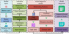 |
Fig. 5 The FDI network structure based on CRDAN algorithm. |
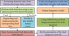 |
Fig. 6 The FDI process of considering FDE and CRDAN algorithm. |
3 Results
To validate the performance of the research design FDE and FDI methods, the study has set up the experimental environment, experimental dataset, and experimental parameters. The study also selects the comparison methods of FDE model and FDI model and analyzes them in terms of accuracy and time consumption (TC).
3.1 Performance validation of FDE method
To validate the performance of the FDE method designed by the study, the study uses Windows 10 operating system with Intel Core i5-12600KF as the central processor with a processor frequency of 3.7 GHz and supports a maximum memory of 128 GB. GPU acceleration was not used to simulate the actual deployment conditions of the embedded platform of the in car Battery Management System without a dedicated graphics card. Test batch size = 16, using single sample inference mode. For the dataset, the experiment uses NASA's publicly available lithium battery dataset, with a total size of 1200 time-series samples and a sampling frequency of 1 Hz [20]. The dataset includes four typical fault types: short circuit, overcharge, overdischarge, and capacity decay, as well as normal state data. The data is divided into training set, validation set, and testing set in a ratio of 7:1:2, without additional data augmentation, to ensure the authenticity of the data distribution.
To verify the effectiveness of the proposed method, 1D CNN, BiLSTM, SVM, SVM + Random Forest (combination model 1), and BiLSTM + Extreme Learning Machine (combination model 2) were selected for comparison in the fault detection stage. 1D CNN uses one convolutional layer, 32 filters, SELU activation function, and max pooling method. BiLSTM is a bidirectional LSTM structure with 64 hidden units. SVM adopts radial basis kernel function with default parameter configuration. Combination model 1 is based on SVM as the classifier, with 100 random forest trees and using a voting fusion strategy. Combination model 2 uses BiLSTM to extract temporal features and extreme learning machine to complete classification. The number of hidden layer nodes is 128. This article presents the convolutional kernel 32 of 1D CNN BiLSTM with SELU activation, Dropout = 0.5, and the maximum number of iterations is 200. Meanwhile, the learning rate (LR) of all models is 0.001, and the opt imizer is Adam. The comparison of FDE accuracy and TC of different models on NASA lithium battery dataset is shown in Figure 7.
In Figure 7a, the maximum values (MaxV) of 1D CNN-BiLSTM, 1D CNN, BiLSTM, SVM, combination model 1, and combination model 2 are 97.53%, 83.51%, 88.23%, 85.09%, 90.33%, and 92.45%, respectively, for the comparison of accuracy. The FDE accuracy of 1D CNN-BiLSTM-M is significantly greater than the comparison model. In Figure 7b, on the comparison of TC, the better performance is the 1D CNN-BiLSTM-M designed by the study. Its MaxV is 71 ms and minimum value (MinV) is 49 ms. Meanwhile, the MaxVs of TC of the five comparison models are 129 ms, 137 ms, 101 ms, 89 ms, and 82 ms, respectively, which are all larger than the TC of the 1D CNN-BiLSTM-M. The comparison model error is mainly due to the incomplete feature extraction of a single model and the lack of adaptive modeling capability of traditional machine learning. The model in this paper combines the advantages of one-dimensional CNN and BiLSTM to effectively reduce the error caused by feature loss and timing modeling deviation. In summary, the research design FDE model has better performance and can detect the faults of EV BPs faster and more accurately. The study itself additionally gathers the pertinent EV BP data in order to further validate the effectiveness of the research design detection model. Furthermore, EVs are mainly sourced from recruitment, after which they are verified by means of manual re-inspection. Therefore, Figure 8 compares the detection precision and root mean square error (RMSE) of several models based on the data gathered for the investigation.
In Figure 8a, the 1D CNN-BiLSTM-M still holds a clear advantage in the comparison of model detection precision. Its MaxV is 98.03%. It is 15.67%, 11.07%, 13.57%, 8.75%, and 5.04% larger than the MaxVs of 82.36%, 86.96%, 84.46%, 89.28%, and 92.99% of the five compared models, respectively. In Figure 8b, on the comparison of model RMSE, the MaxV of 1D CNN-BiLSTM-M is 0.752, and the MinV is 0.004. Meanwhile, the MaxVs of RMSE of the five compared models are 2.985, 2.553, 1.987, 1.230, and 1.107, which are larger than that of the 1D CNN-BiLSTM-M. In conclusion, the FDE model that was created for the study performs better on the real EV BP FDE. Table 1 compares the F1 scores and recalls of various models based on the data gathered for the study.
In Table 1, the better performance in terms of F1 score is the 1D CNN-BiLSTM-M designed by the study. Its average value is 0.985, which is 0.141, 0.100, 0.071, 0.054, and 0.037 higher than the average values of 0.844, 0.885, 0.914, 0.931, and 0.948 of the five comparative models, respectively. Meanwhile, in terms of recall, the one with a higher average value is still the 1D CNN-BiLSTM-M, which takes a value of 98.64%. In summary, the 1D CNN-BiLSTM-M has better performance.
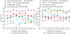 |
Fig. 7 Comparison of FDE accuracy and TC among different models. |
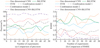 |
Fig. 8 Comparison of detection precision and RMSE of different models. |
Comparison of F1 scores and recall rates for different models.
3.2 Performance validation of FDI method
The Intel Core i5-12600KF central processor and Windows 10 operating system are also used in the study to verify the effectiveness of the research design FDI approach. In terms of dataset, the study follows the data used in FDE, and the processing method was also consistent. The comparative model for fault diagnosis includes SVM, Transformer, SVM + improved whale optimization algorithm (combination model 3), LSTM + autoencoder + K-nearest neighbor algorithm (combination model 4). SVM adopts RBF kernel function and is directly used for multi class fault classification. Transformer has 2 encoder layers and 4 attention heads. Combination model 3 uses classification accuracy as the fitness value, iteratively optimizes to obtain the optimal SVM parameters, and then trains the fault classification model with the optimal parameters, with a population size of 30. Combination model 4 uses autoencoder denoising, LSTM feature extraction, and K-nearest neighbors to complete the final classification. The autoencoder has a 64 dimensional encoding layer, a 64 dimensional decoding layer, and an activation function ReLU. The number of neighbors is k = 5, and the hidden units of LSTM are 64. This article uses the Adam optimizer to jointly optimize the classification loss and domain adaptation loss in CRDAN. The training is completed through 200 rounds of end-to-end backpropagation iterations, with a batch size of 16. The learning rate of all models is 0.001, with 200 iterations. Figure 9 compares the diagnostic accuracy and area under the curve (AUC) of the various models.
In Figure 9a, in the comparison of AUC, the research design diagnostic model takes the value of 0.987, which is closer to 1. Meanwhile, the AUC of SVM, Transformer, combination model 3, and combination model 4 are 0.803, 0.785, 0.922, and 0.946, respectively. Their are 0.184, 0.202, 0.065, and 0.041 less than 0.987, respectively. In Figure 9b, in the comparison of diagnostic accuracy, the better performance is still the diagnostic model of the study design, which has a MaxV of 98.33%. Meanwhile, the MaxVs of diagnostic accuracy of the four compared models are 88.69%, 81.75%, 91.92% and 93.66%, which are lower than 98.33%. The main source of model errors in comparison is the lack of attention weighting and domain adaptation mechanisms, insufficient utilization of fault features, and weak cross condition generalization ability. In this paper, the CRDAN model effectively reduces classification errors through dual attention and category enhancement. Table 2 compares the RMSE and detection precision of several models on various fault types.
In Table 2, on short-circuit faults, the RMSE of the research design FDI model is 0.005, which is significantly smaller than the comparison model. Meanwhile, on overcharge fault, overdischarge fault, and battery cell capacity fade fault, the RMSE of the research design FDI model still performs better. For example, in the battery cell capacity decay fault, the RMSE of the five comparison models are 0.477, 0.400, 0.205, and 0.167, which are 0.458, 0.381, 0.186, and 0.148 higher than 0.019. In addition, on the detection precision comparison, the research design FDI model takes significantly larger values than the comparison model for short circuit fault, overcharge fault, overdischarge fault, and battery cell capacity fade fault.
To further verify the generalization diagnostic ability of the proposed model for more types of faults, this paper adds two typical faults, temperature anomaly and voltage sensor drift, and calculates the false detection rate and missed detection rate under different faults. The results are shown in Table 3.
As shown in Table 3, for the newly added temperature anomalies and voltage sensor drift faults, the false detection rate and missed detection rate of the CRDAN model in this paper are much lower than those of SVM, Transformer, and two types of combined models. Abnormal temperature is affected by environmental conditions, and the drift characteristics of voltage sensors are highly concealed. Traditional models lack feature enhancement and domain adaptation capabilities, which can easily lead to misjudgments and omissions. The model in this article relies on channel time dual attention and category enhancement mechanism, which can accurately capture weak fault features and effectively suppress diagnostic bias caused by working condition disturbances. In the future, by expanding the sample of multiple environmental conditions and introducing sensor noise compensation algorithms, the false detection and missed detection levels of the two types of newly added faults can be further reduced. Figure 10 compares the memory utilization and TC of FDI for various models.
In Figure 10a, in the comparison of the TC of the models, the one that performs better is the FDI model designed by the study. This is followed by the combination model 4 and combination model 3. The SVM and Transformer models come last. In terms of specific values, the MaxVs of TC for the five models are 66 ms, 98 ms, 103 ms, 128 ms, and 146 ms, respectively. In Figure 10b, in terms of memory usage, the MaxVs of research design FDI model, SVM, Transformer, combination model 3, and combination model 4 are 11.31%, 22.62%, 25.17%, 18.19%, and 14.78%, respectively. In conclusion, the research design FDI model has shorter TC, lower memory footprint and better performance.
Single factor analysis of variance was conducted on the experimental results, and significant differences (p < 0.05) were observed in the accuracy, F1 score, recall rate, and other indicators between the CNN BiLSTM fault detection model and the comparative model in this study. There are significant differences (p < 0.01) in AUC and diagnostic accuracy between the CRDAN diagnostic model and comparison models such as SVM and Transformer, indicating that the performance improvement of our method is not random fluctuations and has statistical reliability.
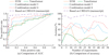 |
Fig. 9 Comparison of AUC and diagnostic accuracy of different models. |
Comparison of RMSE and precision of different models on different types of faults.
False detection rate and missed detection rate under newly added fault types.
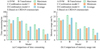 |
Fig. 10 Comparison of FDI time and memory usage among different models. |
3.3 Model interpretability analysis
The interpretability of the CRDAN model in this article is mainly reflected through the physical meaning of attention weights. The specific analysis is as follows: the weight distribution of the channel attention module highly matches the physical characteristics of power battery faults, with the attention weights of the voltage and current channels accounting for 38.2% and 32.7%, respectively, significantly higher than those of the temperature and capacity channels (18.5% and 10.6%, respectively). This is consistent with the physical law that battery faults are often triggered by abnormal voltage and current, indicating that the model can accurately focus on key monitoring signals of faults. The weight of the time attention module is mainly concentrated in the time window of 5–10 seconds before the occurrence of the fault, which can effectively capture the precursor characteristics of the fault such as voltage mutation and current fluctuation, clearly reflect the temporal law of the fault development, avoid the model becoming a “black box”, and improve the credibility and interpretability of the diagnostic results.
3.4 Potential challenges and solutions for actual deployment
Based on the actual operating environment of the in vehicle Battery Management System, the model deployment process may face potential challenges such as sensor errors, environmental changes, and individual differences in batteries. The specific analysis and response plans are as follows:
Sensor error: Vehicle mounted voltage and current sensors are susceptible to electromagnetic interference, resulting in data noise, drift, and other issues, leading to distortion of input model feature data and affecting diagnostic accuracy. Solution: Add an adaptive noise filtering module to the model input, use a sliding average filtering algorithm to suppress high-frequency noise, and introduce a sensor calibration mechanism to correct data drift in real time, ensuring the accuracy of feature data.
Environmental changes: The operating environment of vehicle mounted power batteries is complex, and extreme conditions such as high and low temperatures (−40 °C∼85 °C) and humidity fluctuations can cause the distribution of battery failure characteristics to shift, reducing the model's generalization ability. Response plan: Expand the fault dataset under multiple temperature and humidity conditions, optimize the model domain adaptive module, achieve cross environment adaptive matching of fault characteristics, and improve the robustness of the model in extreme environments.
Individual differences in batteries: Different batches and aging levels of power batteries have significant differences in their fault characteristics, which can easily lead to a decrease in the diagnostic accuracy of the model for new and aging batteries. Response plan: Introduce normalization of individual battery characteristics, establish a universal fault feature library for multiple aging stages and batches of batteries, and fine tune the online model to adapt to the fault diagnosis needs of different individual batteries.
Hardware resource limitations: The hardware resources of the in vehicle embedded platform are limited, making it difficult to support high-speed inference of complex models. Response plan: Lightweight optimization of the CRDAN model, pruning redundant network structures, quantifying model parameters, reducing model memory usage and inference time while ensuring diagnostic accuracy, and adapting to the hardware deployment conditions of the in vehicle Battery Management System.
4 Discussion and conclusion
The study created a 1D CNN-BiLSTM-based FDE model and a CRDAN-based FDI model with the goal of addressing the issue of FDE and FDI of EV BPs. The results indicated that the MaxV of FDE accuracy of 1D CNN-BiLSTM-M was 97.53%. It was 14.02%, 9.30%, 12.44%, 7.20%, and 5.08% higher than the MaxV of 1D CNN, BiLSTM, SVM, combination model 1, and combination model 2, respectively. This might be due to the fact that the model combined the advantages of CNN and BiLSTM to effectively extract local features in the input data and capture temporal dependencies in the sequential data. Meanwhile, this combination enabled the model to understand and analyze the complex patterns in the battery data in a more comprehensive way, thus improving the accuracy of FDE. The AUC of the FDI model was 0.987. It was 0.184, 0.202, 0.065, and 0.041 higher than the AUC of SVM, Transformer, combination model 3, and combination model 4, respectively. Furthermore, the diagnostic model had better diagnostic accuracy and detection precision on different fault types. This could be due to the fact that the model employed a domain-adaptive neural network, which improved the generalization ability (GA) of the model under different conditions. The model adopted both attention mechanisms to highlight important features and suppress irrelevant features. The category enhancement mechanism further strengthened the model's ability to recognize generic fault features, so that the FDI model could recognize and diagnose different types of faults more accurately, thus significantly improving the diagnostic performance. In summary, the research design FDE and FDI models had good performance.
Although the fault diagnosis model proposed in this article has achieved excellent diagnostic results under conventional operating conditions and mainstream battery samples, there are still certain research limitations. On the one hand, the generalization and adaptation of the model to new battery categories such as lithium iron phosphate and solid-state batteries have not been fully validated, and there is still room for improvement in robustness under extremely harsh working conditions such as ultra-high and low temperatures and strong electromagnetic interference; On the other hand, the research only completed the diagnosis of single battery faults and did not deeply consider the identification of cascading faults under the coupling interference of battery pack clusters, and has not yet achieved online incremental iterative updates on the vehicle end. In future research, the study will expand the dataset of battery samples with multiple types and aging levels, as well as extreme operating conditions, and combine cross domain adaptive algorithms to enhance the model's generality. At the same time, the introduction of incremental learning mechanism and graph network topology modeling, taking into account model lightweight optimization, further strengthens the engineering adaptability of the algorithm in complex vehicle environments and new battery systems.
Fundings
The research is supported by: Nanchong Vocational College of Science and Technology General Project in 2024, Development of a Portable Multi-Function Vehicle Fault Diagnosis Teaching Device, (No. XJ2024ZK-39).
Conflicts of interest
All authors declare that they have no conflicts of interest.
Data availability statement
The datasets generated during and/or analysed during the current study are available from the corresponding author on reasonable request.
Author contribution statement
The sole author is responsible for the entire research process, including conceptualization, methodology, software implementation, data interpretation and manuscript writing.
References
- Y. Xu, X. Ge, W. Shen, Adaptive neural observer for short circuit fault estimation of lithium-ion batteries in electric vehicles, IEEE Trans. Power Electron. 39, 1551–1564 (2023) [Google Scholar]
- M. Wu, Y. Sheng, F. Zhang, J. Tang, S. Hu, N. Zhao et al., Fault detection method for electric vehicle battery pack based on improved kurtosis and isolation forest, Int. J. Green Energy, 22, 582–598 (2025) [Google Scholar]
- D.H. Avinash, A. Rammohan, A comprehensive review on advanced fault detection techniques of lithium-ion battery packs in electric vehicle applications, Int. J. Renew. Energy Res. (IJRER), 13, 925–943 (2023) [Google Scholar]
- X. Liu, M. Wang, R. Cao, M. Lyu, C. Zhang, S. Li et al., Review of abnormality detection and fault diagnosis methods for lithium-ion batteries, Autom. Innov. 6, 256–267 (2023) [Google Scholar]
- J. Yuan, S. Li, X. Fan, Sensor fault diagnosis modeling of lithium-ion batteries for electric vehicles, Mater. Express, 13, 875–886 (2023) [Google Scholar]
- S. Sepasiahooyi, F. Abdollahi, Fault detection of new and aged lithium-ion battery cells in electric vehicles, Green Energy Intell. Transp. 3, 42–53 (2024) [Google Scholar]
- J.W. Shen, C. Yan, Y. Liu, Battery fault diagnosis and anomaly detection based on data mining and big data analysis, Trans. China Electrotech. Soc. 39, 7979–7994 (2024) [Google Scholar]
- W. Kim, K. Na, K. Choi, A current sensor fault-detecting method for onboard battery management systems of electric vehicles based on disturbance observer and normalized residuals, Int. J. Control Autom. Syst. 21, 3563–3573 (2023) [Google Scholar]
- M.N. Xia, A fault diagnosis method for electric vehicle charging circuit based on artificial intelligence recognition, J. Comput. 35, 209–224 (2024) [Google Scholar]
- J. Xie, G. Wang, J. Liu, Z. Li, Z. Wei, Faults diagnosis for large-scale battery packs via texture analysis on spatial-temporal images converted from electrical behaviors, IEEE Trans. Transp. Electrific. 9, 4876–4887 (2022) [Google Scholar]
- Y. Xu, X. Ge, W. Shen, A novel set-valued sensor fault diagnosis method for lithium-ion battery packs in electric vehicles, IEEE Trans. Veh. Technol. 72, 8661–8671 (2023) [Google Scholar]
- P.P. Groumpos, A critical historic overview of artificial intelligence: issues, challenges, opportunities, and threats, Artif. Intell. Appl. 1, 197–213 (2023) [Google Scholar]
- X. Li, X. Gao, Z. Zhang, Q. Chen, Z. Wang, Fault diagnosis and detection for battery system in real-world electric vehicles based on long-term feature outlier analysis, IEEE Trans. Transp. Electrific. 10, 1668–1679 (2023) [Google Scholar]
- H.A. Duy, T. Srisongkram, Bidirectional long short-term memory (BiLSTM) neural networks with conjoint fingerprints: application in predicting skin-sensitizing agents in natural compounds, J. Chem. Inf. Model. 65, 3035–3047 (2025) [Google Scholar]
- S. Harishkumar, R.S. Bhuvaneswaran, Enhanced DGA detection in Botnet traffic: leveraging N-Gram, topic modeling, and attention BiLSTM, Peer-to-Peer Netw. Appl. 18, 1–20 (2025) [Google Scholar]
- Z.Q. Ling, J.C. Chen, G.Z. Cao, Y.P. Zhang, L.L. Li, W.X. Xu et al., A domain adaptive convolutional neural network for sEMG-based gait phase recognition against to speed changes, IEEE Sens. J. 23, 2565–2576 (2022) [Google Scholar]
- W. Cheng, L. Chen, W. Wang, A time-frequency domain adaptive impedance matching approach based on deep neural network, IEEE Antennas Wirel. Propag. Lett. 24, 202–206 (2025) [Google Scholar]
- H. Liu, S. Yu, X. Wang, Mega-constellation satellite maneuver forecast via network with attention mechanism, Adv. Space Res. 75, 4942–4962 (2025) [Google Scholar]
- Y. Gao, M. Tian, D. Grana, Z. Xu, H. Xu, Attention mechanism-assisted recurrent neural network for well log lithology classification, Geophys. Prospect. 73, 628–649 (2025) [Google Scholar]
- J.C. Huang, M.H. Shu, H.T. Lin, J.D. Day, Transformer-based lithium battery fault diagnosis research for electric vehicles, J. Intell. Fuzzy Syst. 46, 9329–9341 (2024) [Google Scholar]
Cite this article as: Lichao Wu, Fault detection and diagnosis of electric vehicle battery pack combining neural network and CRDAN algorithm, Int. J. Metrol. Qual. Eng. 17, 16 (2026), https://doi.org/10.1051/ijmqe/2026012
All Tables
Comparison of RMSE and precision of different models on different types of faults.
All Figures
|
Fig. 1 Charging and discharging process of power lithium battery. |
| In the text | |
|
Fig. 2 The structure of battery FDE model based on 1D CNN-BiLSTM. |
| In the text | |
|
Fig. 3 The training and detection process of the battery FDE model. |
| In the text | |
|
Fig. 4 The structure of the channel AM. |
| In the text | |
|
Fig. 5 The FDI network structure based on CRDAN algorithm. |
| In the text | |
|
Fig. 6 The FDI process of considering FDE and CRDAN algorithm. |
| In the text | |
|
Fig. 7 Comparison of FDE accuracy and TC among different models. |
| In the text | |
|
Fig. 8 Comparison of detection precision and RMSE of different models. |
| In the text | |
|
Fig. 9 Comparison of AUC and diagnostic accuracy of different models. |
| In the text | |
|
Fig. 10 Comparison of FDI time and memory usage among different models. |
| In the text | |
Current usage metrics show cumulative count of Article Views (full-text article views including HTML views, PDF and ePub downloads, according to the available data) and Abstracts Views on Vision4Press platform.
Data correspond to usage on the plateform after 2015. The current usage metrics is available 48-96 hours after online publication and is updated daily on week days.
Initial download of the metrics may take a while.