| Issue |
Int. J. Metrol. Qual. Eng.
Volume 15, 2024
|
|
|---|---|---|
| Article Number | 6 | |
| Number of page(s) | 30 | |
| DOI | https://doi.org/10.1051/ijmqe/2024003 | |
| Published online | 25 April 2024 | |
Research article
Application of maximum statistical entropy in formulating a non-gaussian probability density function in flow uncertainty analysis with prior measurement knowledge
Department of Mechanical, Bioresources and Biomedical Engineering, University of South Africa, Private Bag X6, Florida 1710, South Africa
* Corresponding author: This email address is being protected from spambots. You need JavaScript enabled to view it.
Received:
24
October
2023
Accepted:
27
February
2024
Abstract
In mechanical, civil and chemical engineering systems the accuracies of flow measurement instruments is conventionally specified by certified measurement capabilities (CMCs) that are symmetric, however it is physically possible for some flow instruments and equipment to exhibit asymmetric non-Gaussian behaviour. In this paper the influence of non-Gaussian uncertainties is investigated using direct Monte Carlo simulations to construct a probability density function (PDF) using representative non-Gaussian surface roughness data for a commercial steel pipe friction factor. Actual PDF results are compared and contrasted with a symmetric Gaussian PDF, and reveal inconsistencies in the statistical distributions that cannot be neglected in high accuracy flow measurements. The non-Gaussian PDF is visualized with a kernel density estimate (KDE) scheme to infer an initial qualitative shape of the actual PDF using the approximate locations of the normalized peaks as a initial metrologist estimate of the measurement density. This is then utilized as inputs in a maximum statistical entropy functional to optimize the actual non-Gaussian PDF using a nonlinear optimization of Lagrange multipliers for a mathematically unique PDE. Novelties in the present study is that a new methodology has been developed for statistical sampling from non-monotonic non-Gaussian distributions with accompanying Python and Matlab/GNU Octave computer codes, and a new methodology for utilizing metrologist's expert prior knowledge of PDF peaks and locations for constructing an a priori estimate of the shape of unknown density have been incorporated into the maximum statistical entropy nonlinear optimization problem for a faster and more efficient approach for generating statistical information and insights in constructing high accuracy non-Gaussian PDFs of real world messy engineering measurements.
Key words: Pipe flow friction uncertainty / Monte Carlo / non-Gaussian / statistical entropy / optimization
© V. Ramnath, Published by EDP Sciences, 2024
 This is an Open Access article distributed under the terms of the Creative Commons Attribution License (https://creativecommons.org/licenses/by/4.0), which permits unrestricted use, distribution, and reproduction in any medium, provided the original work is properly cited.
1 Introduction
1.1 Research motivation
In mechanical, civil and chemical engineering systems the accuracies of flow measurement instruments is conventionally specified by certified measurement capabilities (CMCs) that are symmetric, and are typically modelled as Gaussian, rectangular or Student's t-distributions. For most practical industrial problems knowledge of an expected value µ and an estimate of an equivalent standard deviation σ, usually estimated via a standard uncertainty σ = u(x), is sufficient to model the statistical distribution via an appropriate symmetric Probability Density Function (PDF), with the use of the Kline and McClintock uncertainty analysis technique [1] that is now a standardized engineering uncertainty method.
On the other hand, for contemporary scientific metrology problems in many national metrology institute and commercial calibration laboratories the Guide to the Expression of Uncertainty in Measurement that is commonly simply abbreviated as the GUM [2], offers more measurement accuracy refinements. These refinements occur where a Gaussian PDF is replaced with a Student's t-distribution through an appropriate calculation of an equivalent degrees-of-freedom veff which allows for the “width” of the PDF to be refined.
These refinements are utilized in calibration certificates and laboratory inter-comparisons in order to more accurately incorporate the statistical dispersion of the tails of a Gaussian distribution and to incorporate correlation effects via covariance matrices for nonlinear measurement models as discussed by Ramnath [3] which generalized and extended earlier work by Kang et al. [4] and Ramnath [5] for the special case of linear statistical regression model parameter uncertainties. More advanced correlation models that extend the concept of covariance matrices include the use of parametric and non-parametric models that incorporate linear error sources and non-linear error sources through the use of a squared exponential covariance matrix function as reported by Tang et al. [6]. These more complex higher order correlation models may sometimes be necessary in high accuracy measurement science work when traditional covariance matrices for linearised multi-physics models such as coordinate measuring machines which incorporate a mixture of mechanical, electrical and optical sub-systems as reported by Habibi et al. [7] and Habibi et al. [8] are insufficient. By contrast, when little detailed uncertainty information is available such as simply a best estimate of a range of values x ∈ [a, b] at a confidence level of say 95%, then under these circumstances an appeal is made to maximal statistical entropy arguments by Bretthorst et al. [9]. Under this scheme that was subsequently adopted by the GUM, the approach is to instead simply model the underlying PDF as a rectangular distribution.
Particular examples according to the GUM for non-Gaussian symmetric PDFs that may be approximately converted to equivalent symmetric Gaussian PDFs include that of a rectangular PDF with a half-width interval a i.e. for x ∈ [− a, b] which may be approximately converted to an equivalent Gaussian PDF by setting  or for a symmetric triangular PDF with a half-width interval of α which may be converted by setting
  such that x ∼ fG(x) = N(0, σ2) with appropriate shifts/translations if the expected value µ is not centred at zero, under the assumption that the underlying PDF is appropriately scaled and normalized such that
  . Examples of the application of asymmetric PDFs utilized in recent engineering research work include the application of the Weibull distribution as studied by Kohout [10] in materials testing work and by Liu et al. [11] in rolling bearing life work, and the Rayleigh distribution as studied by Rezaei and Nejad [12] for the effect of wind speed distribution on wind turbine loading and life duration. Technical limitations with the use of Weibull and Rayleigh distributions center on their lack of general flexibility in modelling the extent of the skewness and kurtosis.
The challenge with the above approaches is that it may physically be possible for some instruments, equipment and measurement systems to exhibit non-Gaussian behaviour that cannot be adequately modelled by symmetric Gaussian, Student's t-distribution, rectangular, Weibull or Rayleigh distributions.
This phenomenon has been investigated by Possolo [13] who reported on asymmetrical measurement uncertainties which were encountered in half-life radioactive decays, astronomical measurements, the absorption cross-section of ozone in atmospheric physics, chemical purity measurements, and banking financial inflation forecasting predictions. Rather than “symmetrizing” asymmetric uncertainties, i.e. by fitting a symmetric uncertainty envelop that is sufficiently broad to encompass the asymmetries by “over-estimating” the uncertainty in order to be conservative so that there is a built in safety-factor in the estimate for the measurement uncertainty, Possolo [13] instead investigated and recommended alternatives to directly modelling asymmetries through the use of the Fechner distribution, the skew-normal distribution, and the generalized extreme value (GEV) distribution. A technical limitation with these proposed distributions is they cannot be readily adapted to PDFs that exhibit double or even multiple peaks, and this presents a current research gap in metrology uncertainty analysis work.
At the present time of writing the state of the art in scientific metrology uncertainty encompasses the use of the GUM and the GUM Supplements which may be considered as specific special cases of a more generalized Bayesian statistics uncertainty analysis as reported by Forbes [14]. An early example of such a Bayesian statistics approach applied to a metrology uncertainty problem was reported by Burr et al. [15] who implemented a Bayesian statistics formulation as an alternative to a more commonly utilized Markov Chain Monte Carlo (MCMC) approach for determining the covariance matrix in a least-squares straight line statistical regression. It is anticipated that future revisions of the GUM in the next decade will incorporate a more mathematically rigorous Bayesian statistics theoretical framework for metrologists working at national metrology institutes and national measurement laboratories.
1.2 Research objective
In this paper, the research objective is to perform an investigation to study the influence of asymmetric non-Gaussian PDF uncertainties on flow measurement systems which exhibit multiple peaks of pipe wall surface roughness measurements which cannot be readily modelled through skewed unimodal distributions, and to examine how these effects influences the performance and measurement accuracies of hydraulic frictional factors in pipes in order to address this research gap in flow metrology asymmetric and non-Gaussian uncertainty analysis. An additional research objective, is to develop appropriate mathematical tools that may be utilized to incorporate prior measurement knowledge in optimizing the construction of an asymmetric non-Gaussian PDF.
1.3 Research approach
The research approach utilized in this paper, is to first perform a literature review of the available statistical theory in Section 2.1 to understand the current limitations in non-Gaussian PDFs for measurement uncertainty. Then in Section 2.2 a review of the corresponding literature for the fluid mechanics of pipe friction flow models is conducted to summarize the available level of scientific knowledge.
After the literature review is completed, in Section 3.1 the mathematical justification of how to combine two different data sets of PDFs of experimental measurements using the technique of statistical conflation is outlined for the physical flow measurement problem that is considered in this paper. Then in Section 3.2 the method of maximal statistical entropy is summarized with relevant formulae, which completes the mathematical formation of the research problem.
Numerical simulations are then performed in Section 4.1 to implement a statistical conflation of non-Gaussian pipe surface roughness data sets that synthesizes the data into a single statistically coherent dataset. In Section 4.2 a new statistical sampling method for performing statistical draws from a non-Gaussian PDF is mathematically derived. An algorithm implementation for the new statistical sampling scheme is also developed. The algorithm is implemented with software code written in Python and Matlab/GNU Octave and the software routines are Validated and Verified (V&V'ed). Data from the non-Gaussian pipe surface roughness measurements are then utilized in Section 4.3 as inputs for the Colebrook mathematical model of a pipe friction factor, by sampling from the PDFs and using these statistical samples in Monte Carlo simulations in Section 4.4. The Monte Carlo data is then post-processed with a Kernel Density Estimate (KDE) algorithm to construct the final non-Gaussian PDF of the pipe friction factor. In Section 4.5 a new approach to incorporate a priori knowledge from a metrologist is developed that may then be used as an input into the Maximum Statistical Entropy (MaxEnt) method, to refine the PDF from statistical moments that are calculated from the Monte Carlo based cumulative distribution function (CDF). The MaxEnt method is then implemented with all of the earlier calculation steps in Section 4.6, and the results are analysed where a flowchart summarises the overall methodology.
Finally, in Section 5 the results are discussed, and conclusions are reported. In Section 6, the influences and implications in point form are summarized.
2 Literature review
2.1 Statistical theories
A Gaussian probability density function (PDF) fG(x), a Student's t-distribution PDF fS(x), or a rectangular PDF fR(x) where x is a random variable, µ is an expected value, σ is a standard deviation where σ2 is a corresponding variance, υ is a number of degrees of freedom, and Γ(Z) is the Gamma function defined as  for a complex argument z ∈ ℂ if Real(z) > 0, are all commonly and presently utilized symmetric PDFs that take the following forms:
 (1)
(1)
 (2)
(2)
 (3)
(3)
For measurement uncertainty work the PDF will be a convenient tool to perform an analysis, where for a univariate distribution with a random variable x the corresponding PDF f(x) is defined such that  where the cumulative distribution function is
  . A multivariate distribution for the joint probability density function for random variables x1, ..., xn in an n-dimensional space ℝn is defined such that Pr[x1, ..., xn ∈ D] = fDf(u1, ..., un)du1...dun where D ⊂ ℝN is a some subset of random variable points within the domain. The corresponding cumulative distribution function (CDF) is defined in terms of the PDF as
  by standard statistical theory.
If a PDF is defined then the distribution may be analysed in terms of the expectation  where E[x] denotes a statistical expectation, the variance is σ2 = V[x] = E[(x-μ)2] where σ is a standard deviation, the skewness is
  , and finally the kurtosis is
  . A majority of algebraic distributions limit the fit to these four parameters as typically only the expectation, variance, skewness and kurtosis have physical meaning in experimental measurements, and to make the analysis more tractable. Additional higher order statistical central moments defined as uk = E[(x − u)k], , which differ from raw non-central moments defined as un = ∫ xxnf(x)dx, are statistically valid but are however not generally considered in existing metrology work since in addition to not typically having any direct physical experimental meaning they are also not generally possible to experimentally measure.
In earlier work by Possolo [13] the use of the Fechner distribution, the skew-normal distribution, and the generalized extreme value (GEV) distribution were proposed as possible distributions to model univariate asymmetries. The Fechner distribution denoted as SN(u, σ1, σ2) is also known as the two-piece normal, binormal or double Gaussian distribution as reported by Wallis [16] and has a PDF of the form
 (4)
(4)
The above distribution has three real parameters, namely a mode value µm (the mode µm is distinct and not equal to the expected value µ), a left-hand-side standard deviation σ1> 0, and a right-hand-side standard deviation σ2 > 0. A multivariate version of the Fechner distribution has been proposed by Villani and Larsson [17] for a p-dimensional random variable x ∈ ℝp which is referred to as a q-split normal distribution SNp(μ, Σ, τ, Q). At the present time of writing there does not exist any generally accepted statistical distributions in analytical form that can conveniently model multiple peaks with varying levels of skewness in metrology uncertainty analysis work beyond these bimodal PDFs which can model only moderate forms of asymmetric skewness, and this presents a research gap in contemporary engineering measurement research.
An alternative more modern skew-normal distribution was originally developed by Azzalini and Capitanio [18] for a k-dimensional random variable z1,…,zk such that z ∼ SNk(Ω, a) where A is a non-singular k×k matrix such that ATΩA is a correlation matrix Σ and a is a vector of parameters. Computations with an Azzalini skew-normal distribution may conveniently be performed with a software library developed by Azzalini [19] in the R statistical computing language. Building on the earlier work of Azzalini and Capitanio a newer form of a multivariate alpha skew Gaussian distribution was subsequently developed and reported by Ara and Louzada [20].
In a different technical approach from the above reported work, asymmetric distributions may also be modelled with extended lambda distributions (ELDs). The use of ELDs in metrology work was originally in a simpler classical form reported by Willink [21] and then in later more powerful forms such as the extended generalized lambda distribution (EGLD) forms as reported by Acar et al. [22], Corlu and Meterelliyoz [23], and Noorian and Ahmadabadi [24] amongst other researchers. Computational statistical libraries such as the EGLD package have been developed by Wang [25], and later a generalised lambda distribution GLDEX package has been developed by Su et al. [26]. Another possibility for modelling asymmetric distributions is to utilize a generalized extreme value (GEV) distribution where the PDF takes the form
 (5)
(5)
In the above formula the set of curves is technically only strictly mathematically valid for  if ξ > 0, and then for
  ξ < 0 where the random variable is x and the transformed variable s is defined as
  where u is a location parameter which is not equal to the mean and σ is a positive scale parameter. The GEV distribution essentially combines the Gumbel, Frechet and Weibull distribution families into a single synthesized distribution that combines characteristics of these underlying constituent distributions. Further theoretical details for generating GEVs are reported in more technical detail by Muraleedharan et al. [27].
Although Fechner, skew-normal families of varying configurations, ELDs, EGLDs, GLDs and GEVs distributions of varying complexities all have their respective merits for modelling asymmetric distributions, a key technical limitation is that all of these approaches inclusive of even newer ones such as generalized Marshal-Olkin transformation based distributions reported by Klakattawi et al. [28], are all fundamentally restricted to uni-modal single peak distributions and cannot incorporate multiple peaks when fitting an underlying statistical distribution.
If a PDF exhibits multiple peaks then a fit that is only able to incorporate a single peak with varying levels of skewness, would essentially produce a PDF envelope that is sufficiently broad to “over-fit” the underlying PDF, but which would over-estimate the associated uncertainty. This phenomenon of utilizing simplified forms of PDFs has been observed to occur when performing a GUM based uncertainty analysis where the Gaussian or Student's t-distribution for the PDF approximation has been observed to be significantly “fatter” when compared to a more accurate Monte Carlo constructed PDF that is more “narrow” to the extent that an over-fitted symmetric PDF that can envelope the actual PDF introduces unrealistic and inaccurate predictions of the actual measurement uncertainty.
In principal, a copula as originally proposed by Possolo [29] may be used to model an arbitrary univariate or multivariate distribution inclusive of non-Gaussian and/or multiple peak behaviour. At the present time of writing, the use of copulas is more widely known and utilized in scientific metrology uncertainty analysis work, than models such as the squared exponential covariance matrix by Tang et al. [6] as discussed earlier, since copulas can theoretically model arbitrary levels of higher order covariance effects with appropriate choices of copulas and marginal distribution functions. Particular examples of the latest research in copula theory, include the use of the empirical beta copula as discussed by Segers et al. [30], and the use of the empirical Bernstein copula and the empirical checkerboard copula as discussed by Lu and Ghosh [31]. This approach of using copulas has previously been applied by Ramnath [32] for bivariate models with weakly non-Gaussian distributions of the form f(x1, x2) = F(x1)G(x2)C(F(x1), G(x2) ; θ) where F(x1) = μ and G(x2) = ν are marginal cumulative distributions which may be modelled with quantile functions (QFs) or with ELDs of varying complexity.
Copulas when used to model PDFs utilize a function c(F(x1), G(x2) ; θ) that is known as a copula density which is calculated as  and where C is the copula function and θ = (θ1, ..., θq) is an appropriate copula parametrization factor based on the choice of a copula family that models the coupling effect between independent random variables, and is usually done from a selection of parametrized families of copulas based on optimizations in standard statistical software packages. As a result for most practical cases when fitting copulas to a PDF the information for the value of q is relatively small and it is common to use a single parameter with q =1 or at most three or four parameters so that θ = (θ1) or θ = (θ1, θ2, θ3) for example, and to retain more complexity in the marginal distributions. A challenge for constructing a wholly analytical approach is to select appropriate parametrizations of the marginal distributions once the optimal copula density is optimized. The use of copulas generally requires a very large number of Monte Carlo simulation events in order to accurately fit an appropriate copula model.
Originally the modelling of marginal distributions for univariate distributions was analytically solved through the fitting of extended lambda distributions through the calculation of statistical moments as proposed by Harris et al. [33]. When this approach was investigated it was concluded by Ramnath [32] that this method is sufficiently accurate for weakly non-Gaussian univariate or multivariate marginal distributions that have asymmetries with single peaks. In the particular case where there is a strongly non-Gaussian behaviour, a mixed analytical/numerical approach may be used that incorporates an analytical form for the copula density whilst a pure numerical calculation of the marginal distributions through empirical cumulative distributions for F(x1 and G(x2) may be used.
A proposed approach for a wholly analytical construction of a PDF or a joint PDF to avoid non-parametrized empirical distributions may be achieved by following the earlier work by Harris et al. [34] to utilize a quantile function constructed as a polynomial B-spline function of sufficiently high order and associated number of knots to model the underlying behaviour of either a univariate or marginal distributions with a vector parameter θ that contains the terms for the fitting of a B-spline.
For most practical metrology problems, particularly for high accuracy scientific metrology work in national measurement primary standard scale realizations and commercial industrial calibration laboratories, to achieve a meaningful quality of fit with splines for arbitrarily complicated “messy” functions would typically require anywhere from 100 to 1000 data points, however a fundamental limitation with even a very high order polynomial is that of Runge's phenomenon, which tends to introduce artificial oscillations near the end-points of the interpolated domain. A practical alternative to mitigate against the Runge phenomenon is the use of splines as discussed earlier by Harris [33] who addressed this technical issue with the use of B-splines.
Whilst the use of B-splines as a linear combination of piece-wise basis functions is an improvement on the use of oscillatory polynomials or cubic splines, there may nevertheless still be an excessive number of parameters associated with the spline knot locations and parameters. The earlier work by Ramnath [32] also exhibits a technical limitation in terms of the unimodal single-peak nature of the fitted PDF, even when asymmetry and skewness can be modelled may be modelled with more complex non-Gaussian models such as the Fechner or GEV distributions, and thus a suitable compromise between the number of parameters and an ability to model multiple peaks in distributions is desirable.
If a suitable alternative method could be developed to accommodate multiple possible peaks with a more manageable number of fitted parameters and non-monotonic behaviour is possible, then this approach when adopted with a wholly analytical model for a PDF f(x) where x = (x1, ...xn) may instead be constructed through a set of curves for each of the underlying marginal distributions F1(x1) = μ1, ..., Fn(xn) = μn with independent parametrizations θ1, ..., θn for each of the fitted curve terms. In general the length of θi may or may not be equal to the length of θj for i≠j, and then an analytical copula C(µ;θ) where μ = (μ1, ..., μn) and Θ = (Θ1, ..., Θm) is another vector of parameters of suitable length m, may instead be used to conveniently model the coupling effects which may exhibit asymmetry and multiple peaks.
Whilst a fully analytical model for constructing a univariate PDF or joint PDF for a multivariate distribution may be appealing or desirable, in practical terms this would in general result in an excessive and unnecessary number of parameters. A more practical solution if the underlying statistical data is available through for example Monte Carlo simulations as discussed by Smith et al. [35] and Armstrong [36] when pre-processing the statistical data, is to directly utilize the available numerical data with either an empirical beta copula as discussed by Segers et al. [30] or alternately through a kernel density estimate approach as discussed by O'Brien et al. [37] when post-processing the statistical data. These approaches are conceptually powerful and simple enough to apply for arbitrary distributions including highly non-Gaussian distributions, avoid unnecessarily complicated fitting of equation parameters, have readily available computational implementations, but however all require a large number of Monte Carlo simulation events which is not always feasible in particular types of experiments in some metrology laboratories.
A useful approach when analysing the post-processed data when non-Gaussian behaviour for the PDF is present and appropriately modelled, is to utilize Rosenblatt transformations to decompose the marginal distributions as discussed by Ramnath [38] such as when conditional PDFs must be calculated when performing a measurement uncertainty analysis when some of the PDF inputs are known or constrained.
2.2 Fluid theories
Fluid mechanics problems in engineering utilizes the concept of a friction factor λ in pipe flow which is only mathematically present on the boundary conditions of a fluid/solid interface such as a pipe wall, as internal fluid friction within the fluid is fully mathematically accounted for from knowledge of the fluid dynamic absolute viscosity µ.
Although a microscopic boundary condition such as the surface roughness may be considered to not have a very significant effect on the overall performance of a macroscopic system a recent investigation by Khanjanpour and Javadi [39] who performed Computational Fluid Dynamics (CFD) studies to investigate the effect of surface roughness on a Darrieus Hydro (DH) turbine concluded that a surface rough height variation of up to 1000 µm increased the turbulence and decreased the active fluid energy, to the extent that a turbine's overall drag coefficient was 20% higher than a smooth turbine blade with a zero roughness height. This study thus demonstrated that microscopic surface roughness effects can have significant macroscopic equipment and instrument consequences in flow measurement equipment accuracy, particularly in metrology pressure and flow systems where laboratory instrument accuracies must typically range from a fraction of a percent to several parts-per-million. A recent review by Kadivar et al. [40] reports on the current state of experimental and theoretical knowledge for fluid flows over general rough surfaces, and it is anticipated that Direct Numerical Simulation (DNS) work will become increasingly common in CFD based simulation studies of surface roughness effects in pipes.
In the special case of pipe flows Ludwig Prandtl, widely considered to be the father of modern aerodynamics, originally performed a mathematical analysis to account for friction data in terms of an explicit equation of the form  where
where  is the Reynolds number for a pipe with a hydraulic diameter of d, V is the pipe bulk flow velocity,
  is the fluid kinematic viscosity, µ is the fluid dynamic viscosity, and ρ is the fluid mass density. An approximate alternative to the implicit form for λ includes the well known Blasius equation
  which may be considered as an approximation to the more accurate Prandtl equation for a more limited range of Reynolds numbers.
Experimental work by Charles-Augustin de Coulomb discovered that the pipe wall surface roughness directly effected the value of the friction however this effect is considered negligible for laminar pipe flow when the Reynolds number is relatively small. At higher Reynolds numbers with rough surfaces for a fully rough flow the friction equation developed by Nikuradse takes the form  where ϵ is representative wall roughness height and (ϵ/d) is known as the dimensionless roughness ratio.
The physical difference between a fully rough regime and a transitionally rough regime is essentially dependent on the prevailing Reynolds number. For low Reynolds numbers where the fluid velocity is small the effect of the viscosity is more dominant and will tend to damp out disturbances caused by the localized surface roughness and this flow regime is categorized as hydraulically smooth. On the other hand, as the fluid velocity increases then so to does the Reynolds number, and with this flow regime the induced turbulent eddies near the pipe surface are not fully damped by the viscosity, and so the drag caused by the shape of the irregularities on the surface tends to contribute more to the overall drag. At a certain value of Reynolds number the drag becomes dominant and this flow regime is referred to as fully rough. Thus a pipe flow regime varies from hydraulically smooth, to transitionally rough to fully rough, and this is correlated to the prevailing Reynolds number.
These earlier historical fluid mechanics experimental studies were subsequently utilized by Colebrook [41] to cover the transitionally rough range by combining the hydraulically smooth wall model of Prandtl and the fully rough model of Nikuradse into a single interpolation formula for the pipe friction in the transitional rough regime of the form
 (6)
(6)
The above implicit non-linear Colebrook formula for the pipe friction λ where ϵ is also known as an equivalent sand grain roughness corresponding to the diameter of a grain of sand, is now generally considered to be the accepted universal engineering design formula to directly compute the turbulent friction factor in a pipe with appropriate numerical routines implemented in software packages such as Fortran or Matlab.
Different schemes exist that attempt to correlate the equivalent sand grain roughness height ϵ, also written as ks to signify the Nikuradse sand grain size, with the surface roughness height statistical data as shown in Figure 1. One particular algorithm to estimate the equivalent sand grain roughness developed by Adams et al. [42] is  .
.
Alternative schemes reported by Shockling et al. [43] for the arithmetic average is  and for the root-mean-square (RMS) is
  , where
  is the fluctuation which may be positive or negative of the profile surface roughness height relative to the mean height
  of the pipe wall corresponding either to a ‘peak’ or ‘valley’, and where L is a suitable interval of measurement to provide a reasonable estimate of the surface roughness properties. Typical spot sizes for surface roughness measurements in this study on selected regions on the pipe wall are 0.8mm×1.2mm, and typical values for the arithmetic and RMS averages for steel pipes are Ra ≈ 0.116μm and Rq ≈ 0.15μm.
The application of the above formula for Ra by Adams et al, or alternative competing schemes, to implement the algorithm assumes that xy profile data from longitudinal x scans of the surface height y along the surface are available, such that for a small interval along the surface the arithmetic average of absolute values Ra is calculated, where  is the mean line of the height and
  is the difference between a measured point on the surface and the mean line, and the corresponding value of the equivalent sand grain roughness ∊ is solved from the integral equation. In this manner the value of ϵ may be conveniently calculated from arbitrary surface roughness xy profile measurements of the pipe surface. At the present time of writing there does not exist a unique universally accepted method to convert geometrical roughness measurement quantities such as Ra or Rq into an equivalent Nikuradse sand grain size ϵ=ks, although recommendations such as that by Hama [44] propose that for machined surfaces with an approximately Gaussian variation in roughness that ks ≈ 5krms whilst more recent studies by Zagarola and Smit [45] suggest that for honed and polished surfaces that ks ≈ 3krms.
In the original study by Colebrook [41] for the data with transitional roughness the equation took the form  where ks is the equivalent Nikuradse sand-grain roughness value for the pipe inner wall surface and λ is the friction factor that is defined in terms of the pipe flow pressure gradient
  the pipe inner diameter D, the fluid mass density ρ, and the center-line bulk velocity
  as
as  .
.
A graphical alternative to the Colebrook equation is the well known Moody chart which is accurate to approximately ±15% and is commonly used in many engineering design studies for initial scoping designs for both circular as well as non-circular pipe flows. An alternative explicit formula developed by Haaland [46] which has an accuracy of ±2% approximates the implicit Colebrooke equation as
 (7)
(7)
Once the pipe friction factor λ has been determined the subsequent analysis of pipe networks flows may be performed based on the work of Jeppson [47] as a branch of hydraulic engineering at the interface of mechanical, civil and chemical engineering. These calculations are typically performed by using knowledge of λ to calculate the equivalent head loss hf in meters corresponding to a pipe pressure drop caused by the pipe friction factor expressed as a column of water for the length L of the pipe using the formula 1.
 (8)
(8)
When the surface roughness of a pipe has a known PDF for the value of ϵ as pϵ(ξ) then this uncertainty information may be propagated into the measurement model for λ in order to produce a corresponding PDF gλ(η) that models the uncertainty variation of the pipe friction factor, which may be Gaussian or possibly non-Gaussian, and which in turn may then be used to calculate the uncertainty in the equivalent head loss hf with a PDF ghf(ξ), that can then finally be used in quality engineering studies for investigating the reliability of pipe flow network systems.
Subsequent fluids research work by McKeon et al. [48] investigated fully developed turbulent pipe flow data in the range 31 × 103 ≤ Red ≤ 35 × 106 and utilized a generalized logarithmic law in order to combine the high Reynolds flow data with earlier low Reynolds flow data in the Blasius equation in order to construct a new equation for the friction that is accurate to ±1.4% for the entire low/high Reynolds flow data and which agrees with the Blasius model at low Reynolds numbers to within ±2.0%, where the new equation for the friction term λ= f is accurate to ±0.002 and takes the form of an implicit non-linear equation  .
.
Shockling et al. [43] studied the effects of roughness for turbulent pipe flow for fully developed flow with experimental data in the high Reynolds range 51 × 103 ≤ Red ≤ 21 × 106 and concluded that the traditional Moody diagram for the friction is inaccurate in the transitionally rough regime and should be used with caution. Their investigation demonstrated that in the transitionally rough regime that the friction factor follows a Nikuradse type of inflectional relationship rather than the monotonic Colebrook type of behaviour based on a Buckingham π dimensional analysis which proved that the friction factor follows a functional relationship such that  where π1 is an unknown functional that must be determined. Later experimental work by Allen et al. [49] with Reynolds data for 57 × 103 ≤ Red ≤ 21 × 106 confirmed an inflectional relationship for the friction factor instead of the expected monotonic behaviour predicted from the traditional Moody diagram and which validated the Townsend outer-layer similarity hypothesis for rough walled pipe flows.
Afzal [50] analysed friction factor data from the available literature and investigated the influence of roughness parameters including the arithmetic mean roughness Ra, the roughness mean peak to valley height Rz, the root-mean-square (RMS) value of roughness Rq, the ratio Rq/H where H is the surface texture Hurst parameter, and h is the traditional equivalent sand grain roughness value. This study concluded that the pipe friction factor λ can be modelled with the Prandtl smooth pipe friction factor equation provided that the traditional Reynolds number Re is instead replaced by a new roughness Reynolds number defined as  where ϕ is a new non-dimensional roughness scale. Different types of formulae were found to be necessary for various roughness scales and may be summarized in terms of the equivalent sand grain roughness h for fully rough and transitionally rough pipes as
  for fully rough and
  for transitional rough flows.
The above fluid theories for modelling the pipe friction factor may then be incorporated into Computational Fluid Dynamics (CFD) based simulation studies of flow measurement equipment and instruments such as that by Wang et al. [51] who investigated an elbow flow meter, and that by Gace [52] who investigated a Coriolis Mass Flowmeter (CFM), where the friction factor λ affects the CFD boundary conditions. These CFD studies would incorporate reference liquid density measurements of actual oils and associated working fluids that have measurement traceability back to an appropriate national metrology institute as discussed by Akcadag and Sariyerli [53].
 |
Fig. 1 Geometry of pipe inner wall surface roughness measurements scheme illustrating positive amplitudes in peaks and negative amplitudes in valleys in Nikuradse equivalent grain size diameter experiments. |
3 Mathematical modelling
3.1 Synthesizing Independent PDFs
Techniques for mathematically combining independent measurements that are modelled with PDFs as continuous distributions is an emerging area of metrology research with the increased adoption of the Monte Carlo based uncertainty approach of the GUM Supplement 1 [54] for univariate measurements and the GUM Supplement 2 [55] for multivariate measurements. At the present time of writing there is no widely accepted methodology within the metrology field to uniquely combine independent PDFs of measurement distributions as the existing techniques are orientated for combining discrete measurements.
Particular methods for combining independent discrete measurements include the use of weighted arithmetic averages in terms of Graybill-Deal statistical estimators for a sequence of independent measurements {x1, x2, ..., xn} of a measurement y where the expected value of y is then calculated as  with an estimated uncertainty u(y) calculated as
  as discussed by Ramnath [56] for experiments. An alternative is the application of the standard methodology for computing a key comparison reference value (KCRV) from multiple independent laboratory measurements as reported by Cox [57]. The existing methods for combining discrete measurements are only technically valid in the special case that each of the individual estimates independent measurements {x1, x2, ..., xn} follow an underlying Gaussian distribution i.e.
  or equivalently can be reasonably approximated with a Gaussian distribution. If the underlying discrete measurements cannot be approximated with Gaussian distributions then weighted means will produce inconsistent and statistically inaccurate estimates of the consensus value of x and its associated uncertainty µ(x). Whilst individual laboratories at various national metrology institutes in their primary and working standards may utilize the GUM supplements to generate an accurate prediction of the measurement PDF, these calculations at present have to be approximated as Gaussian PDFs in order to utilize this uncertainty information in inter-laboratory comparisons.
Current research by Willink [58] for combining two independent PDFs has investigated the subtle inconsistencies from a Bayesian statistics framework that may potentially arise when combining two independent PDF estimates of a single quantity. To illustrate the logical inconsistencies which may arise if for example two PDFs p1(x) and p2(x) representing independent sets of information about an unknown quantity are available, then this knowledge may be synthesized and combined into a single unique PDF for the unknown x as  . This formula is a special case where the measurand is given by the linear equation y = x and the probability of the measurement output is the same as the model input so that formally py(η) ∼ gx(ξ) using standard metrology uncertainty analysis from the GUM. It is known to be mathematically correct and consistent in the special case where there are two or more independent PDFs that directly specify knowledge for a single quantity x that does not have any significant functional dependencies on other additional measurement quantities and may therefore be directly utilized to correctly combine the surface roughness PDFs later in this paper.
Clemen and Winkler [59] report on an interesting possible use of copulas for combining expert knowledge of a parameter θ by synthesizing the independent PDFs fi(θ) with corresponding CDFs Fi(θ) so that the posterior distribution is  . In this above equation θ(x) denotes some parameter which depends on x, and c[u1, ..., un], where u1 = 1 − F1(θ), ..., un = 1 − Fn(θ) denotes the copula density function outlined in an earlier metrology study by Ramnath [32]. Clemen & Winkler report that a potential benefit of the use of copulas for synthesizing independent expert judgements is that the individual expert judgements for the final parameter θ are entirely separate from any underlying dependence characteristics which are made separately and directly encoded into the copula density function.
3.2 Maximum statistical entropy
The original formulation of the principle of maximum statistical entropy to the PDF problem was by Mead and Papanicolaou [60] who utilized the fundamental equation  , with n ∈ ℕ that links a univariate PDF P(x) where x. is a random variable to the statistical raw moments
  . Later work by Bretthorst [9] revisited the original problem by comparing the methods of binned histograms in multiple dimensions, kernel density estimation, and the method of maximum entropy of moments in an earlier attempt to synthesis or combine the two different competing approaches of the maximum entropy (MaxEnt) and the Bayesian statistics formulation for determining the optimal probability density function.
More recent work by Armstrong et al. [36] has succeeded in developing a more advanced mathematical new hybrid method that combines the maximum entropy and Bayesian statistics competing approaches for estimating the optimal PDF in the particular case where there is limited knowledge of the statistical moments or when there is noisy data that pollutes the accuracy of the statistical moments. This newer method, simply termed the MaxEnt/Bayesian approach for brevity, is applicable to large scale real world engineering problems where it is infeasible and in some cases simply impractical with available technology to adequately generate a very large number of Monte Carlo simulation events.
The PDFs generated with the MaxEnt/Bayesian approach can theoretically be refined and made more accurate as newer information on the a priori PDFs becomes available by incorporating the newer measurement uncertainty information into the Bayesian scheme using a Metropolis algorithm with a Markov Chain Monte Carlo strategy (MCMC/Metropolis) as discussed in more technical detail by Armstrong et al. [36].
In the particular area of scientific metrology the measurement uncertainty problems at the present time of writing are typically of a much smaller scale albeit at a significantly higher scientific accuracy level with less statistical noise when compared to measurement problems encountered within industry. As a result the maximum statistical entropy method is generally more appropriate for metrology work at primary scientific standards level than the MaxEnt/Bayesian method. For many representative applications work in mechanical, civil and chemical engineering in various metrology fields it is usually possible to generate a sufficient number of Monte Carlo simulations with modern physical multi-core laptops/workstations or rented virtual cloud computing services such as the Amazon Elastic Compute Cloud (Amazon EC2) service that are amenable to deploying open source codes such as OpenFOAM as discussed by Jahdali et al. [61] that can then be used to accurately calculate a sufficient number of statistical moments.
Under these conditions, using the standard calculus integration by parts formula ∫udv = uv − ∫ vdu and noting that the PDF f(x) may equivalently be defined as  with the CDF F(x) it then follows noting that F(xmin) = 0 and F(xmax) = 1 by definition from statistical theory, that the corresponding raw statistical moments μn for a measurement model output random variable η is then just
 (9)
(9)
In the above formula the actual CDF F(η) in the definition of the statistical moment µn may be conveniently approximated with an empirical cumulative distribution function (ECDF) that does not require any knowledge of the PDF. The zeroth moment  is automatically known to be unity from standard statistical theory. The GUM Supplement 1 [54] provides a simple piece-wise interpolating formulae for the underlying discrete approximation G(η) with the actual Monte Carlo data Ω.
A useful benefit of computing the statistical moments in terms of the CDF instead of the PDF is that integration is well known by mathematicians to “smooth out” numerical noise and this provides a very convenient and useful numerical strategy to avoid the more difficult problem of calculating derivatives of noisy data encountered later in this paper.
Once the raw statistical moments µn are known, the principle of maximum statistical entropy approaches the determination of the PDF by maximizing the Boltzmann-Shannon entropy function defined as S[f(x)|m(x)] ≔ − ∫ x∈xf(x)ln[f(x)/m(x)]dx where m(x) contributes as an invariant measure. Armstrong et al. [36] report that S[f(x)|m(x)] is actually equal to the negative of the Kullback-Leibler divergence, which means in practical terms that the statistical entropy provides for a mathematical technique to determine the optimal PDF. This is achieved by formulating an equivalent Lagrangian function using the earlier approach of Mead and Papanicolaou [60]. Omitting the theoretical details for brevity, the final result for computing the unknown PDF f(x) is then
 (10)
(10)
 (11)
(11)
In the above formula x is the random variable and X is the space in which x resides, λn are unknown Lagrangian multipliers which must be solved for from knowledge of statistical moments µn, and Z is essentially a type of normalization constant to ensure mathematical and statistical consistency. For a univariate PDF if the limits of x are a ≤ x ≤ b then X=[a,b] is just the closed interval on the real line. Spaces for X which is the domain in which x resides in may be extended to higher dimensions for x ∈ ℝn = ℝ × … × ℝ. Although the “shape” or topology of X in higher dimensional spaces may possibly be irregular in non-Gaussian PDEs in most practical cases X will conservatively be constrained either to correspond to a hyper-ellipsoidal region if the PDF is roughly Gaussian or alternatively to a higher-dimensional rectangular box in ℝn to be conservative if the PDF is non-Gaussian as outlined earlier by Ramnath [62]. The invariant measure m(x) is an initial approximation to f(x) and the MaxEnt approach provides for a way to incorporate the estimate m(x) in a unique equation, where λn are unknown real parameters technically known as Lagrange multipliers which must be solved for. Mead and Papanicolaou [60] mathematically proved that the Lagrange multipliers may be uniquely determined by minimizing the free energy defined as
 (12)
(12)
 (13)
(13)
The presence of the natural logarithm of the partition function term ln(Z) in the above formula necessitates an unconstrained nonlinear optimization in higher dimensional spaces  as the number N of the Lagrange multipliers increases.
4 Numerical simulations
4.1 Synthesizing non-Gaussian input PDFs
Experimental data for a pipe surface roughness ϵ = ks reported by Shockling et al. [43] and later Langelandsvik et al. [63] both demonstrate a distribution that exhibits multiple distinct peaks as shown in Figure 2 that demonstrate a distinctly non-Gaussian PDF for a pipe friction factor flow measurement uncertainty analysis, which suggests that the pipe friction factor λ may also exhibit a non-Gaussian PDF.
The earlier data by Shockling et al. has a spread of ±8 μm whilst that by Langelandsvik et al. has a spread of ±15 μm. The physical interpretation of a positive value of grain size with ks ≥ 0 is that this value of ks occurs above the mean value of the surface i.e. is a peak amplitude, whilst a negative value of grain size with ks ≤ 0 occurs below the mean value of the surface i.e. is a valley amplitude.
Physically in any fluid pipe flow measurement the equivalent grain size ks will always be non-zero, thus in order to perform an analysis it is therefore necessary to first post-process the bimodal PDF data in order to avoid a negative value of ks. This can be conveniently achieved by taking the absolute value of the surface roughness data so that positive amplitudes measured as peaks above the mean surface remain unaltered whilst negative amplitudes measured as valleys below the mean surface become equivalent positive roughness values. In this manner, two sets of experimental roughness data, one for the roughness amplitudes above the mid-surface and another for the roughness amplitudes below the mid-surface, may be obtained for the pipe surface roughness profiles. This set of experimental datasets can then be synthesized with only the absolute surface roughness value of ks as only positive values of ks is mathematically valid in the Colebrook equation and has a physical meaning in a fluid dynamics analysis for calculating a pipe friction factor λ. Referring to the graph in Figure 2 it may be observed that each of these constituent PDFs are clearly asymmetric distributions and must be combined in a mathematically consistent manner. By taking only the absolute values of the surface data for each of the datasets by Shockling et al. [43] and Langelandsvik et al. [63] the two independent PDFs may be generated as shown in Figure 3.
Letting  and
and  denote the corresponding valley roughness data and peak roughness data for the Shockling et al. dataset, with random variables ξv and ξp for the valley and peak surface roughness variables, it follows that from the previous section that these two individual PDFs may then be combined as
  to yield a single combined PDF that obeys the normalization condition
  , with a similar expression
  for the combined Langelandsvik et al. dataset.
The mathematical notation &(P1,P2) for combining two or more PDFs P1 ∼ f1(ξ), P2 ∼ f2(ξ) into a single PDF is termed conflation following the earlier work by Hill [64] where the conflation is mathematically defined as  This conflation formula by Hill is an earlier special case of the later more general analysis by Willink [58].
 |
Fig. 2 PDFs of the inner wall surface roughness for commercial grade steel pipes reported by Shockling et al. [43] and Langelandsvik et al. [63]. |
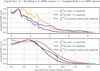 |
Fig. 3 Comparison of equivalent PDFs of the peak and valley amplitudes reported by Shockling et al. [43] and Langelandsvik et al. [63]. |
4.2 Statistical sampling from a non-Gaussian PDF
For the pipe surface roughness amplitude measurements it may be observed that both of the resulting combined PDFs from the Shockling et al. and Langelandsvik et al. data-sets are both clearly not Gaussian PDFs. It may also be observed that both datasets exhibit asymmetry whilst only the Shockling et al. dataset demonstrates multiple peaks. The corresponding cumulative distribution functions (CDFs) are shown in Figure 3 from which a technical challenge posed by the multiple peaks and skewness may be observed. In a monotonic PDF curve the standard technique to sample from the underlying distribution is to generate a random number between zero and unity that follows a rectangular distribution and to then read off the corresponding random variable ξ from the CDF curve since 0 ≤ F(ξ) ≤ 1 by definition. For symmetric Gaussian PDFs the corresponding CDF is always monotonic in a graph of the CDF for F(ξ) versus ξ data points and it is straightforward to perform an interpolation for monotonically increasing data points.
By contrast the key technical difficulty and technical implementation issue which results due to the combination of asymmetry and multiple peaks in non-Gaussian PDFs, is that a single random number, say 0.43 in the Shockley et al. curve FS(ξ) = 0.43 represented by the dashed orange line, would yield multiple possible values ξ1 ≈ 2.3μm, ξ2 ≈ 2.6μm, ξ3 ≈ 2.8μm of the corresponding random variable ξ that can all technically simultaneously solve the equation F(ξ) = 0.43. A similar non-monotonic behaviour also occurs in the Langelandsvik et curve FL(ξ) = 0.02 represented by the dashed magenta curve where possible solutions are ξ ≈ 2.2μm, ξ ≈ 4.1μm, ξ ≈ 4.6μm. When performing a Monte Carlo simulation an arbitrarily large number of multiple roots would also occur near F(ξs) = 0.43 e.g. 500 random points for 0.42 ≤ F(ξS) ≤ 0.45 and similarly say 250 random points near 0.01 ≤ F(ξL) ≤ 0.03. This non-unique sampling problem would be exacerbated with noisy data with multiple maxima/minima. This is considered to be a unique metrology uncertainty problem which has not been previously encountered, and does not appear to have been previously solved and reported within the available technical and scientific literature.
The key mathematical challenge which arises in sampling from a non-Gaussian cumulative distribution function is therefore the presence of multiple roots for the nonlinear function F(ξ) which is caused by the presence of multiple maxima/minima. In general, a non-Gaussian CDF may exhibit multiple maxima/minima for a corresponding range 0 ≤ F(ξ) ≤ 1 of random variables ξmin ≤ ξ ≤ max and it is not appropriate to “smooth out” these fluctuations as it would cause a sampling bias, noting that there is a fundamental difference in smoothing noisy statistical data and eliminating physically meaningful surface roughness amplitude variations that may be physically caused by peculiarities in machining and surface grinding of metallic pipes and other machined components.
The presence of multiple physically meaningful maxima/minima in the CDF curve causes a horizontal line to intersect the CDF curve multiple times. When a graph of F(ξ) of the vertical/ordinate data versus the ξ horizontal/abscissa data is plotted to determine a corresponding value of the random variable ξ from a specified value of F(ξ) = r this would then generate a non-monotonic curve. Standard numerical interpolations in software such as Matlab and Python all require a single x value and a single y value to make an interpolation in a curve y = f(x) unambiguous otherwise such a numerical routine would automatically fail. If a numerical routine only selects either a first or last value for a y value from a specified x value, from multiple possible values of y, this would then automatically introduce an artificial systematic bias when attempting to sample points from a non-Gaussian distribution. When sampling from a non-Gaussian distribution the x values correspond to F(ξ) which is assumed known and the y values correspond to ξ which is considered unknown and must be inferred. The problem of non-monotonicity is that a single x value allows for multiple y values.
Noting that a random rectangular variable r∼R[0,1] may take an infinite number of possible values, there are then a very large number of possible intersections between a horizontal line with a constant value of r which may cut the curve F(ζ) at varying levels, and that may have several maxima/minima along the axis where the random variable lies. This fundamental statistical problem of sampling from a non-Gaussian distribution in this paper is proposed by mathematically reformulating it as finding all multiple roots for the nonlinear function ϕ(ξ) defined as
 (14)
(14)
A straightforward attempt to solving the above problem by searching for all points where ϕ(ξ)is such that ϕ(ξ)< TOL can provide a rough initial estimate may be achieved by iterating through a discrete set of the pairs  however the specification of the magnitude of the tolerance TOL is a subjective decision and would logically vary on a case by case basis in different measure uncertainty experiments leading to a mathematically ill-posed problem. An incorrect specification of TOL could then unintentionally result in under or over estimating the number of roots i.e. the number of intersections of a curve r=const and F(ξ) that lie in an envelope of possible solutions for ϕ(ξ). If the incorrect number of multiple possible roots is solved by under counting or over counting the roots by an incorrect specification of TOL, then the corresponding set random variables that solve F(ξ) = r would introduce a systematic statistical sampling bias and lead to erroneous measurement uncertainty predictions for non-Gaussian systems.
This technical complexity of multiple roots in a non-Gaussian sampling is not present in a traditional Gaussian sampling approach where the data is monotonic. If the PDF is symmetric then the CDF would almost always be monotonic unless there is an extreme level of skewness present. Under the assumption of a monotonic data for F(ξ) versus ξ curve it is straightforward to sample in language such as Matlab or GNU Octave with the code fragment r=r and(), xival=interp1(Fdata − r, xidata, 0). This simplifying assumption of monotonic data would not apply for a CDF with multiple peaks, and a new computer sub-routine for numerically interpolating in non-monotonic data curves corresponding to statistical sampling from non-Gaussian distributions must instead be developed.
The lack of monotonicity in the CDF due to the non-Gaussian multiple peak nature of the distribution may theoretically solved by parametrizing the curve into piece-wise smooth segments that have the same gradient sign such that the CDF is the union of these individual sequential segments so that
 (15)
(15)
Referring to the PDF data in Figure 3 which may be post-processed to calculate the CDF in Figure 4 using the standard statistical formula  where ξ is simply a dummy variable for performing the integration, it may be observed that when the gradient of F(ξ) changes from positive to negative a localized maxima occurs, or alternately when the gradient changes from negative to positive that a localized minima occurs. This geometrical change of gradient is the source of the non-monotonicity which would cause a conventional interpolation routine to fail, and suggests a convenient geometrical solution, namely to “simply break up the non-monotonic curve into a sequence of sequential segments which are each individually monotonic” in order to possibly take advantage of existing interpolation routines which work on monotonic data curve.
When decomposing a “messy” curve into a sequence of piece-wise smooth curve segments, a simple approach to avoid spurious maxima/minima peaks from noisy oscillations that artificially generate additional peaks is to use a Savitzky-Golay filter to smooth out the signal in the curve as shown in Figure 5 which uses a window length of 11 and a smoothing polynomial of order 5 with a nearest neighbour selection of points on either side to damp out fluctuations for the particular problem of pipe surface roughness and pipe friction factor examined in this paper. The particular parameters for filtering/smoothing signals would in general vary on a case by case basis in other metrology problems.
To sample from the smoothed/filtered non-Gaussian distribution would then involve the generation of a random variable r from a rectangular distribution r ∼ R[0, 1] and then selecting an appropriate segment Sj from the set of all sequential segments S1,S2,…,SN that has a range such that  . In this scheme, it is still technically possible for two or more different segments who may occur in different parts of the domain to each have a range that includes the sampled value r, i.e. it is technically possible to have multiple possible solutions to the equation F(͠ξ)=r in different regions of the domain as shown in Figure 6 which illustrates the fundamental mathematical complexity with non-Gaussian PDFs in a metrology uncertainty analysis.
The numerical strategy in this paper is to perform a sample from all of the possible segments and to then select all of the corresponding feasible value of ξ is considered to be theoretically valid if the sequence of segments are smooth and continuous. Continuity in the case of imperfectly constructed segments for the CDF F(ξ), can be enforced by joining discontinuous segments either with straight lines or with arcs that match the values and slopes of the segments on either side of the discontinuity such that no vertical segments in any discontinuous F(ξ) is present. The need for an absence of vertical segments joining discontinuities in a F(ξ) curve is because the PDF is defined as  and the derivative of a vertical line would be undefined and lead to a mathematically inconsistent PDF.
Whilst this approach of decomposing a complicated curve with multiple maxima/minima into a sequence of simpler curves that do not exhibit localized peaks/troughs, avoids an additional sampling bias when performing a Monte Carlo simulation as it is relatively simple to randomly sample from a large number of events, it is more challenging to generate a sequence of random integers if for example 3 possible values ξ1,ξ2,ξ3 can all simultaneously solve F(ξ)=0, j=1,2,3. This situation would occur if a horizontal line cuts across three different segments. Choosing all possible values that solve F(ξj)=0 avoids the unnecessary complexity of generating random selections of integers to select from the available three choices of solutions, and also ensures that the simulation remains physically valid as technically all equivalent sand grain sizes in the roughness amplitude are physically possible.
Practical technical challenges with this proposed approach of partitioning the non-monotonic curve as a sequence of constituent monotonic curves includes that finding the exact point ξ at which the gradient  is zero based on discrete data can be technically challenging, particularly in cases where the slopes are nearly horizontal with zero gradient and which makes it difficult and ambiguous to uniquely estimate the intersection of the segments without accounting for the numerical resolution error.
In addition to the above technical challenges with a theoretical solution of the non-monotonic interpolation problem, from a practical implementation point there may also be a very large number of segments to construct particularly if there are a large number of multiple maxima/minima in the CDF curve. This phenomena is illustrated in Figure 7 where the Shockley et al. PDF previously shown has a total of 14 local minima/maxima peaks for the range of possible random variable ξ.
The corresponding peaks are first obtained by taking the gradient  and solving for the roots by checking where the gradient changes sign from positive to negative or alternately from negative to positive to estimate an approximate first estimate that can then be refined. If there are 14 roots r1,…,r14 that solve the equation ϕ(ξ)= 0 then there are 14-1=13 interior sub-segments to consider which when combined with the two segments on either side of the lowest root for ξmin ≤ r1 and highest root for r14 ≤ ξ ≤ ξmax then produces a total of 13+2=15 segments S1,…,S15 where Sj = { (ξi, F(ξi)) } , j = 1, ..., n. When sampling in order to solve ϕ(ξ) = F(ξ) − r would then require first checking whether each of these 15 segments contains a possible solution by testing if the random value lies in the range min(F(ξ)) ≤ r ≤ max(F(ξ)) and then solving the equation. If the non-Gaussian distribution is “messy” and contains many maxima/minima then the number of segments to convert a non-monotonic curve into an equivalent sequence of monotonic curves can quickly become numerically infeasible.
Taking the above technical issue into consideration, a practical work-around solution proposed in this paper to resolve these technical and mathematical issues that can be conveniently and quickly implemented in Python with the numpy library in this article is as follows:
In the above computer code fragment, the basic numerical strategy is to fit a B-spline as a set of piece-wise smooth polynomial functions to the irregular F(ξ) data and generate this curve for a very large number of points comparable to the number of Monte Carlo simulation events. In most physical experimental work at scientific metrology level at NMIs and commercial calibration laboratories the typical minimum number of Monte Carlo simulation events in an uncertainty analysis is usually in the range from M = 15 × 103 to M = 100 × 103 to meaningfully approximate the underlying measurement uncertainty behaviour and characteristics. As a result curve fitting for irregular curves that cannot be adequately modelled with analytical Gaussian or weakly non-Gaussian distributions comprising of a few hundred thousand points is usually feasible on most modern laptops with sufficient memory and processing speed.
Once the data is generated which exhibits the non-monotonic behaviour i.e. a single value of F(ξ) which may have multiple solutions of ξ, the standard Python search function where may then be applied on numpy arrays in order to determine the array indices just before the array is zero. As an example if a Python array is z = np.array([–0.63, −0.4, 0.2, 0.56]) which has indices [0,1,2,3] then the index position just before the array value is zero corresponds to element at index 1 which signifies that the zero-crossover point is in-between the values for calculated as v = np.where(np.diff(np.signbit(z)))[0] will have the location at index 1 because there is only sign change from negative to positive (or alternately from positive to negative). This index search on the array elements is achieved by testing the sign of all the elements in the array with the signbit function which yields a Boolean True if the array element is negative and the diff function which checks where there exists a difference in the sequential Boolean values i.e. by checking if the next element has a Boolean False corresponding to a positive element. Where a difference of Boolean True and Boolean False values exist, or vice versa, then this index logically corresponds to a value just before zero. The specific value at which a zero occurs is still unknown but the index search is considered to be sufficiently accurate to provide an initial estimate where a zero occurs in an array which may have 15000 to 100000 elements. If the number of elements becomes very large then this allows for the spatial resolution of the zero cross point to be refined. The approximate value at which the zero actually occurs may also be estimated from a linear interpolation of the values.
In the limit as N becomes very large the index of the point just before the value is zero is thus then seen to be approximately coincident with the point where it is actually zero if equally spaced points are used in an interpolation such as a B-spline or a univariate spline. The standard Python function can determine multiple instances for the indices just before the array is zero. An example using the Shockley et al. cumulative distribution function data from Figure 4 to demonstrate the accuracy of the proposed method as the number of points N becomes very large with N =15,000 is shown in Figure 6 that exhibits a multiplicity of roots. Referring to this graph, it is observed that when a random value such as r = 0.63 is sampled that the algorithm correctly identifies that the root multiplicity is three and estimates the roots as ξ1 = 2.908, ξ2 = 3.049, ξ3 = 3.179 respectively which is visually verified from the graphical information for accuracy. In a Monte Carlo simulation that requires statistical sampling from non-Gaussian distributions all three values of the random variable that solves F(ξ) = r would be selected, since all three random variables are mathematically and statistically valid.
In the limit as N becomes very large the index of the point just before the value is zero is thus then seen to be approximately coincident with the point where it is actually zero if equally spaced points are used in an interpolation such as a B-spline or a univariate spline. The standard Python function can determine multiple instances for the indices just before the array is zero. An example using the Shockley et al. cumulative distribution function data from Figure 4 to demonstrate the accuracy of the proposed method as the number of points N becomes very large with N =15,000 is shown in Figure 6 that exhibits a multiplicity of roots. Referring to this graph, it is observed that when a random value such as r= 0.63 is sampled that the algorithm correctly identifies that the root multiplicity is three and estimates the roots as ξ1 = 2.908, ξ2 = 3.049, ξ3= 3.179 respectively which is visually verified from the graphical information for accuracy. In a Monte Carlo simulation that requires statistical sampling from non-Gaussian distributions all three values of the random variable that solves F(ξ) =r would be selected, since all three random variables are mathematically and statistically valid.
This example thus demonstrates the intrinsic difference in sampling from a symmetric Gaussian probability density function where there is only one random variable for a particular draw, and in the sampling from an asymmetric non-Gaussian probability density function where there are theoretically multiple possible sampled values which may be associated with a statistical draw. The accuracy of the root estimate from the proposed method in this paper is observed as being sufficiently accurate when a large enough number of data-points are used to fit the B-spline approximation of the CDF.
If a higher accuracy for solving F(ξ)= r is required then this approximate location for ξ may be further refined as necessary by taking several ξ values before and after the estimate of the value of ξ for the zero cross over point instead of a linear interpolation since only discrete points are known and it is not possible to work out the exact value of ϕ(ξ) = 0, by then fitting a quadratic polynomial as ϕ(ξ) = F(ξ) − r = aξ2 + bξ + c which can be conveniently achieved with standard matrix operations.
The above numerical method may also be adapted and generalized if necessary at localized estimates of the multiple roots by choosing other classes and other types of interpolation formula to model curve shapes to approximate F(ξ) if a low order polynomial such as a quadratic or cubic is found to be inadequate. An example of an asymmetric curve is a sigmoidal S-shape with some skewness that may be modelled in the form g(x ; b, c, d, e, f) = c + (d − c)(1 + exp[b { log10(x) − log10(e) } ])−f for log-logistic type of curve with other forms as discussed by Spiess et al. [65].
A statistical sampling from a specified non-Gaussian CDF which may exhibit multiple peaks and varying levels of skewness therefore consists of solving the equation ϕ(ξ) = F(ξ) − r = 0 for a sampled specified value of r for the random variable ξ. The available numerical strategies for solving for the roots of ϕ(ξ) = 0 and hence computing a statistical sampling from F(ξ) in order of increasing accuracy/complexity are then:
An indirect estimate of the zero crossing from a sign change of discrete points ϕ(ξ) as the sign changes from positive to negative or vice versa with a large number of discrete points, i.e. a 0th-order numerical sampling scheme.
A linear interpolation near the zero cross over point from discrete values of ϕ(ξ) which exhibit sign changes, i.e. a 1st-order numerical sampling scheme.
A quadratic polynomial approximation of near the zero cross over point from a few neighbouring discrete points near the zero cross over, i.e. 2nd-order numerical sampling scheme.
The accuracy of all of these numerical strategies essentially depends on the computational accuracy of the B-spline interpolation for generating values of F(ξ) as ϕ(ξ) = F(ξ) − r, as the explicit analytical form of F(ξ) is unknown. A comparison of the the proposed 0th order, 1st order and 2nd order sampling schemes for a non-Gaussian distribution with the Shockley data-set is summarized in Table 1 by examining the Shockley data-set for the non-Gaussian pipe surface roughness where there are three possible repeat roots ξi(i = 1,2,3) i.e. ξ1,ξ2,ξ3 at different parts of the curve for the equation ϕ(ξ) = F(ξ) −r by using values of n=1000,n = 5000 and n = 15000 discrete data-points for the [ξ,F(ξ)] curves to check for relative errors and convergence.
A representative graphical summary of this tabular data is shown in Figure 8 for a sampled random variable corresponding to r= 0.43 and by selecting just the first root ξ1 for convenience. Referring to this graph it is concluded that sampling scheme #1 is inaccurate for a small number of n = 100 discrete points on the non-Gaussian cumulative distribution curve, sampling scheme #2 and sampling scheme #3 are essentially indistinguishable for medium to large numbers of points, and that all three sampling schemes tend to converge for large numbers above n = 15000 discrete points on the CDF curve. As a result, the specific choice of statistical sampling scheme becomes less of a technical issue in the limit of a large number n of discrete points.
From the above discussion where it was demonstrated that there is a convergence for n = 15000 discrete points or larger, the numerical accuracy from a finite number of discrete points when solving for the roots of ϕ (ξ) = 0, under the assumption that F(ξ) can be accurately estimated for specified values of ξ from a B-spline curve fit, can conveniently be reduced by simply using a very large number of points n. A rough estimate for the accuracy of the sampling resolution with the Shockley et al. data-set, has a domain which varies from min(ξS) = 0.034122 to max(ξS) = 8.325840. When searching for roots in the interval, the discrete resolution for points on a uniformly spaced grid is then Δ (ξS) = (max(ξS) − min(ξS))/(n − 1). As a result, the discrete spacing when searching for sign changes of ϕ (ξ) is (8.325840 − 0.034122)/(15000 − 1) so that Δ (ξS) = (5.5278 × 10⁻⁴) = ± 0.0005μm. A similar calculation for the Langelandsvik et al. data-set with min(ξL) = 0.060768 and max(ξL) = 15.161798 yields Δ (ξL) = ± 0.001μm. Thus sampling with strategy # 1 using an underlying curve with n = 15000 fitted discrete points in a simple index search for the roots would have resolution accuracies of ±0.0005μm and ±0.001μm for the non-Gaussian surface roughness Shockley and Langelandsvik data-sets respectively.
The above calculations therefore demonstrates that for a large enough number of discrete points on a cumulative distribution curve, that even if the curve exhibits strongly non-Gaussian and multiple peak statistical behaviour, that the statistical sampling error with numerical strategy # 1 is essentially negligible, and that it would seldom be necessary to utilize the trade-off between the algebraic complexity and increased accuracy that is directly available from either sampling strategy # 2 or sampling strategy # 3.
Technical implementation details for the three developed numerical strategies are summarized at the end of the paper in the Appendix in Figure A1 for a Python code implementation and in Figure A2 for a Matlab/GNU Octave code implementation for sampling for a single scalar value of the random variable r, as extending these codes for sampling with multiple random values r1, … , rM in a typical Monte Carlo simulation that requires M simulation events is straightforward. When performing such a simulation the number of sampled values is not necessarily exactly equal to M due to the possible presence of repeat roots, thus it would usually be advantageous to use an adaptive Monte Carlo scheme. A convenient benefit of statistical sampling with a numerical sub-routine with a single specified value of r is that it simplifies any subsequent quality engineering validity and verification (V&V) work of developed computer codes in metrology laboratories.
Once a statistical sampling from the non-Gaussian surface roughness PDFs has been achieved for the amplitude ε = k values then these random variables may be substituted into the pipe friction model with the Colebrook equation and numerically solved for the friction factor λ.
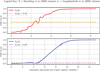 |
Fig. 4 Comparison of CDFs of the surface roughness amplitudes with noise. |
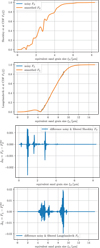 |
Fig. 5 Surface roughness CDFs showing Savitzky-Golay filtering to avoid spurious maxima and minima. |
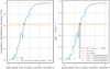 |
Fig. 6 Illustration of multiple peaks producing a multiple root search for a non-Gaussian PDF statistical sampling. |
 |
Fig. 7 Illustration of procedure converting a nonmonotonic curve into a sequence of monotonic curves. |
Summary of proposed discretization scheme accuracies for sampling from a non-Gaussian PDF.
 |
Fig. 8 Graphical summary of the convergence characteristics of the numerical sampling schemes. |
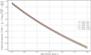 |
Fig. 9 Illustration of a sequence of Colebrook equations with varying random roughness values. |
 |
Fig. 10 Empirical cumulative distributions of pipe friction factor for Shockley and Langelandsvik datasets. |
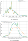 |
Fig. 11 Probability density function curves for Shockley and Langelandsvik input data-sets on the Monte Carlo simulation outputs for the pipe friction factor λ values showing Gaussian, piecewise linear fit of peaks locations/relative values and kernel density estimate to the actual non-Gaussian probability density function. |
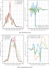 |
Fig. 12 Final simulation results for the probability density function of the pipe friction factor using the maximum statistical entropy method with results for the Shockling and Langelandsvik non-Gaussian surface roughness data-sets. |
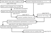 |
Fig. 13 Flowchart summary of main steps to implement a MaxEnt refinement of a non-Gaussian PDF. |
4.3 Solving a nonlinear Colebrook equation
Praks and Brkic [66] investigated a variety of numerical methods to solve the nonlinear implicit Colebrook equation, and examined amongst other approaches iterative schemes based on a simple iterative fixed point scheme, Householder iterative methods, three-point iterative methods, approximations using Artificial Neural Networks (ANNs), and the Lambert W-function approach where the Darcy flow friction factor λ is solved from an equivalent equation  .
.
A direct numerical solution for the Colebrook equation without transformation mappings such as the Lambert W-function, is to instead estimate an initial rough guess λ0. A value for λ0 reported by Prak & Brkic that can achieve convergence after about six iterations with a straightforward Newton-Raphson iterative scheme following Burden [67] is simply the corresponding laminar flow approximation for low Reynolds numbers expressed as  . In order to implement a Newton-Raphson solution with the initial guess λ0, the first derivative for an equivalent homogeneous equation must be explicitly analytically calculated in order to achieve faster convergence over iterative derivative free schemes such as the secant method. Computing the first derivative is algebraically lengthy and technically cumbersome as it involves an implicit partial derivative calculation.
Writing an equivalent homogeneous equation  for the Colebrook equation by using the result that
  so that log10x = ln(x)/ln(10) and by setting
  , 2.51 = C2, ϵ = k, Red = R, and L = λ it follows that
  therefore
  thus
thus  . This homogeneous equation can now conveniently be formulated with the Python symbolic package sympy to work out the corresponding implicit derivative
  as follows:
When the above code is run the partial derivative is then calculated as  The value of the unknown λ in the formula f (λ) = 0 is then solved using a standard Newton's method where the estimate for λ is sequentially estimated for convergence using the initial approximation λ0 and the above derivative
  as
as  .
.
This approach for solving a nonlinear friction factor λ in the Colebrook equation with a starting solution λ0 and a derivative calculated with the aid of a computer algebra system such as sympy, can in principle be adapted and applied to other more complicated pipe friction models such as the Afzal model for pipe transitional rough flows. In the event that the derivative cannot be analytically calculated then derivative free approaches such as the secant method can instead be utilized.
4.4 Monte Carlo simulation of friction factor
To perform a numerical simulation by solving a nonlinear Colebrook equation corresponding to a number of Monte Carlo simulation events, it is necessary to first select appropriate engineering parameters and specifications for a pipe flow problem. Most industrial and municipal steel pipes for large flow network systems would typically have pipe diameters that range from 100mm to 1000mm, and many municipal water pipes for bulk supply have an internal pipe diameter of D = 0.3m as this readily available. A typical municipal water network in a water scarce country such as South Africa can have a pipe network of 8790 km that has 287 pumping stations, 27 waste water treatment plants, and 407500 sewer connections as reported by Friedrich and Kretzinger [68]. This illustrates the underlying scale and engineering significance that pipe friction factors can have as a relatively small change in the friction factor λ in pipes when applied over many kilometres can have significant cumulative engineering and economic consequences, including significant pressure drops and consequent financial implications such as the optimal placement and financial cost of boosting pump installations. A related pipe friction metrology uncertainty problem occurs in the petroleum refinery sector where representative pipe network specifications for a diesel and jet fuel refinery by the state owned enterprise Sasol near the port city of Durban on the eastern coast in the Republic of South Africa that supplies processed petroleum products to inland plants is summarized in Table 2.
Numerical simulations in this paper are therefore performed with a 16-inch pipe so that D = 16 × 25.4 × 10 −3 = 0.4064m, a pipe length of 15 km so that L = 15000m, and a volumetric flow rate of 1100 m3/hr so that  . For these pipe flow specifications since Q = AV is the product of the pipe cross-sectional area
  and the velocity V it follows that the pipe velocity is
  . Taking a heavy diesel kinematic viscosity of 4.1mm2/s so that ν = 4.1 × 10⁻⁶m2s−1 and assuming a mass density of ρ = 845kgm−3 then yields a Reynolds number of Re = VD/ν = (2.3556 × 0.4064)/(4.1 × 10−6) = 2.3349 × 10⁵ which specifies the baseline engineering specifications and parameters for a pipe friction analysis. Since all the parameters in the Colebrook model in equation (6) are specified it is seen that only the pipe wall roughness ϵ = k is free to vary from a specified probability density function. When k is allowed to vary according to the specified density distribution from the previously outlined statistical sampling
  then a sequence of measurement equations η = f (ξ) must be numerically solved as shown in Figure 9 such that the solutions of these equations form the measurement model outputs. Once the measurement models
  are solved then the PDF may be generated.
A summary of the main steps using the above specifications to perform a Monte Carlo simulation using the sampled non-Gaussian pipe surface roughness data to generate a probability density function for the pipe friction factor λ is then as follows:
The underlying non-Gaussian probability density function data reported in Figure 5 for both the Shockley et al. and Langelandsvik et al. data-sets of the pipe surface roughness ϵ with n = 15000 points on the [ξ = ϵ, F (ξ)] curves are sampled using the new method developed in this paper for M = 100000 Monte Carlo simulation events in the previous section by solving equation (14) with statistical sampling strategy #2 with a linear interpolation scheme.
The sampled values with a total number of M⋆ ≥ M due to possible multiple peaks/multiple roots when sampling from the non-Gaussian distribution of the surface roughness ϵ are then substituted as random variables
 into the Colebrook formula in equation (6) and numerically solved using a starting value of λ0 from the Haaland equation with the Newton formula to produce M⋆ Monte Carlo simulation events
The M⋆ Monte Carlo simulation events are post-processed as a univariate statistical data-set
 as M⋆ × 1 vectors using the GUM Supplement 1 methodology to generate the corresponding empirical distribution function GS (ηS) and GL (ηL) corresponding to the Shockley and Langelandsvik surface roughness for the pipe friction factor λ
The distribution functions GS (ηS) and GL (ηL) from the above Monte Carlo simulation are graphically summarized in Figure 10 with a discrete empirical cumulative distribution function (ECDF) where for a specified value of M=100000 draws a total of  and
and  random values were sampled from the Shockley and Langelandsvik distributions respectively due to the non-Gaussian and multiple maxima/minima peaks which introduced multiple roots. This number of Monte Carlo simulation events is considered sufficiently large to accurately calculate the statistical moments at a higher enough order and at a level with a negligible amount of statistical noise. For a smaller specified value of M =15000 the corresponding values were
  and
and  which shows a similar pattern of roughly 37% and 12% extra sampled points in the Shockley and Langelandsvik distributions respectively due to the presence of multiple peaks/multiple roots which occur when sampling from these distributions. The extent of the extra sampled points in arbitrary non-Gaussian PDFs would in general vary based on the particular measurement model's input statistical distribution on a case by case basis.
The corresponding probability density function is directly obtained from the Monte Carlo data using a kernel density estimate (KDE) approximation with the Python based Seaborn statistical package using the default automatic parameters Scott's method when selecting for the appropriate bandwidths and enforcing cut-off of tails beyond the minimum and maxima points in the underlying Monte Carlo data to avoid un-physical values in the tails as shown in Figure 11 for an easy qualitative visualization.
Since the value of M⋆ is very large this PDF will be assumed to specify the model's actual output PDF. As discussed earlier there does not exist any general purpose parametric based non-Gaussian PDF model that can incorporate an arbitrary level of skewness and multiple peak, which is an open research problem. The next section outlines the implementation of the maximum statistical entropy method for constructing the PDE that refines an initial a priori estimate m(x) with knowledge of the statistical moments μn to construct an optimal PDF f(x) that is closer to the true PDF.
Representative engineering pipe flow specifications for a typical petroleum refinery.
4.5 Metrologist a priori knowledge of density
In order to apply the principle of maximum statistical entropy in order to construct the actual probability density using knowledge of the statistical moments it is necessary to have an initial approximation of the density based on an a priori knowledge. This knowledge may come from a metrologist based on prior measurement experience from the equipment and instruments for the experiments, theoretical insights, or partial experimental data points that is insufficient to adequately generate an empirical cumulative distribution function with a sufficient resolution and accuracy due to practical constraints on time, labour, and available financial resources in metrology laboratories. In this paper we will consider two a priori estimates for the density as follows:
a Gaussian approximation based on a rough qualitative estimates for the expected value μ and standard deviation σ.
an approximate piece-wise density based on estimated peaks in the density.
The first approach is documented in standard statistical books as summarized in equation (1) and is commonly utilized instead of a Student's t-distribution summarized in equation (2) when there is little available information such as an effective degrees of freedom veff to either further refine the shape of a symmetric Gaussian density or single peak asymmetric density distributions such as Fechner/skew-normal or GEV density functions.
As discussed earlier, the major challenge with the use of a single peak density function such a Gaussian curve is that this approximation will tend to introduce errors in the predicted uncertainties by making the tails “fatter” when there are multiple maxima/minima that are present in the density of the measurement. In the complete absence of any knowledge of the statistical parameters it is common metrology uncertainty analysis practise to simply assume a rectangular density function as summarized in equation (3). A practical challenge with assuming a rectangular distribution as an initial approximation to m(x) is that a very high number of moments μn would then be necessary as essentially this assumption logically implies that the PDF is then approximated as  . Mead and Papnicolaou [60] remarked that this approach would require a very high number of statistical moments μn that were not polluted by numerical/statistical noise.
In certain measurement based experimental work, although the actual shape of the measurand density may not be possible to construct due to limited information, based on limited experimental data it is nevertheless still possible to estimate localized peaks in the density by the metrologist who performs the physical experiments. This approximate a priori measurement knowledge can for example be obtained from discrete histogram plots and by a qualitative interpretation of the available measurement data from spreadsheets of tabulated measurements.
If in addition to the approximate location of the peaks, the relative frequencies of the peaks of the densities are also known from approximate histograms, then a very approximate piece-wise density function m(x) may be constructed by straight lines to join the expected peaks/valleys as shown in Figure 11. It may be noted that this approach is based on the limited available information so that the resolution on the exact locations and exact numbers of peaks is inaccurate based on the time constraints of physical measurements that take from one to two weeks and produce data-sets that typically have less than 100 points. The utility of the maximum statistical entropy principle in metrology uncertainty work is that as new measurement uncertainty information becomes available, either through repeat calibrations or possibly inter-laboratory comparisons (ILCs), then this additional information may be incorporated to update and refine the probability density function f(x) of the measurement. Referring to the figure of the metrologist a priori estimate of the density curve two practical issues may be observed.
The first issue is that based on the shape that the absolute values of the densities of each of the three curves may widely vary in magnitude which may introduce numerical errors. The second is that the magnitude of the random variable n, in this paper the pipe friction factor λ which is 0.015173 ≤ ηS ≤ 0.015355 for the Shockling data-set and 0.015175 ≤ ηL ≤ 0.015502 for the Langelandsvik data-set, may be either very small or very large depending on the nature of the metrology uncertainty problem. The combination of these issues may result in the physical statistical moments μn being very small as shown in Table 3. Both of these practical numerical issues are resolved in this paper by scaling the magnitudes of the random variable i.e. instead of using x = 0.015355 ≈ 1.5355 × 10⁻² as a random variable which requires powers of x when working out the moments a new scaled random variable is used e.g. x⋆ = 102x ≈ 1.53 so that the numerical errors is reduced. The subsequent mathematical analysis in the next sections may be conducted without any loss of generality as in a measurement uncertainty analysis it is only the shape of the density function which is required as the absolute values of the random variables and the absolute values of the PDFs may be recovered in a straightforward manner.
Summary of raw statistical moments of pipe friction factor.
4.6 Inference of PDFs from statistical entropy
A measurement science challenge with simply using the KDE approximation for the PDF in metrology work in laboratories at national metrology institutes and national measurement laboratories, is that the choice of bandwidth h which for one-dimensional PDFs is essentially analogous to the width of histograms is subjective and ad-hoc, and that in some measurement problems it is simply not possible or infeasible to generate a sufficiently large enough number of Monte Carlo simulation events M to mitigate this issue.
The ad-hoc nature of the KDE bandwidth therefore presents considerable validity issues in the specific area of scientific metrology work where measurement uncertainties that are based on subjective criteria such as the bandwidth are not considered reproducibility and unique, and are thus not universally accepted at a primary scientific standards level. If h is too small then under-smoothing occurs, whilst if h is too large then there will over-smoothing. Particular methods for estimating the KDE bandwidth include rule of thumb methods such as the Scott method with  where
where  is the sample standard deviation or the Silverman method with
  where IQR is the inter-quartile range, and cross-validation methods such as the Maximum likelihood cross-validation (MLCV) discussed by Chen [69].
The Scott method is only accurate for uni-modal densities that are approximately Gaussian whilst the Silverman method is known to produce inaccuracies for more complicated density variations. Theoretical challenges with optimization based approaches such as least squares based cross-validation methods is that the bandwidth selection exhibits a large variation according to sample size as outlined by Chiu [70]. In the present context of flow measurement accuracy work the sample size corresponds to the number of Monte Carlo simulation events in pipe flow systems which may dramatically vary by metrologists working in different flow measurement laboratories. Although the problem of optimal KDE bandwidth is an active and ongoing research area, in the specific area of scientific metrology there is as yet no agreed consensus on the correct choice of KDE bandwidth, and this is not expected to be resolved until a new edition of the GUM [2] is published in the next decade.
The ambiguity in the correct optimal choice of a KDE bandwidth, from a variety of competing approaches, can theoretically be avoided with a sufficiently large number of Monte Carlo simulation events by using an empirical cumulative distribution function from which an empirical probability density function may be calculated that does not require any parameters.
A technical challenge which occurs with directly attempting the construction of the PDF g(η) without any underlying parametrized model from a purely empirical cumulative distribution G(η) by using finite differences to work out  is the presence of numerical noise from the Monte Carlo simulation. In general, to work out the derivative of noisy signal data would require either smoothing with filtering to “de-noise” the data or polynomial/spline interpolation to “smooth out” the noisy function data. Earlier investigations by mathematicians have proved that de-noising of messy data does not necessarily always guarantee smooth derivatives. Both of these approaches thus again present traceability issues for scientific metrology work of primary standards calibrated at high accuracies as the choice of filter or type/order of smoothing interpolation is again also subjective. Alternatives to avoid the problem of derivatives of noisy data include the use of the Total Variation Regularization (TVR) method as reported by Chartrand [71] which uses a functional analysis formulation and optimization, or the use of a fast Fourier transform (FFT) to smooth out noisy signal data as reported by Kosarev and Pantos [72].
Referring to the density shape from the KDE graph in Figure 11 it may be observed that multiple peaks and asymmetry are clearly visible in the pipe friction model outputs from both surface roughness input data-sets, which demonstrates the intrinsic non-Gaussian nature of the flow measurement uncertainty problem studied in this paper. This provides numerical evidence that in general non-Gaussian model inputs when propagated through a nonlinear model tend to produce a model output that is both nonlinear and non-Gaussian. In the graph are also shown a priori estimates of the likely density shape by a metrologist from a combination of measurement expert knowledge and experience based on locations and relative values of peaks/valleys that in this paper provides a qualitative best guess of what the density shape is expected to be as the actual PDF is unknown and it is desired to utilize the statistical moments to refine this estimate.
The particular meaning within a scientific metrology context of a nonlinear model y = f (x1, x2, x3) with say three inputs x1, x2, x3 and a single output is that a linear model can be represented with a linear equation as y = ax1 + bx2 + cx3, i.e. as a linear combination of the inputs, whilst a nonlinear model cannot be represented with this equation, and that the meaning of a non-Gaussian model is that the output of the model y does not follow a Gaussian distribution such that ηy ∼ (μ, σ2) and instead follows some other distribution that cannot be represented with a Gaussian probability density function that is defined entirely with just the two parameters of an expected value μ and a variance σ2.
A similar mathematical formalism may be generalized and used to explain the meaning of nonlinear and non-Gaussian in the case of multivariate input/output measurement models with vectors in a measurand equation y = f (x). Technically the meaning of nonlinear and non-Gaussian are not synonymous and interchangeable, and it is actually mathematically possible to have a nonlinear model that is Gaussian or alternatively a linear model that is non-Gaussian.
From a qualitative inspection of the approximate shape of the PDF from the KDE plots it can immediately be observed that the single peak skew normal and generalized extreme value distributions are both rejected as they can only model a single peak with asymmetry and skewness. A double Gaussian distribution in terms of Fechner PDF can also not exhibit multiple peaks so this is also rejected, in favour of the qualitative best guess of a metrologist from prior knowledge and experience as this incorporates more meaningful insight of the likely shape. This a priori estimate of the PDF is not necessarily inaccurate as it could involve a few more accurate measurements in particular ranges of the random variable ξ which generates detailed knowledge of the location of the peaks but less information of the spread of the peaks.
Ideally knowledge of the both the location and spread of the density peaks is desirable, however credible knowledge of the number of peaks and their locations in an a priori best estimate of the density may possibly be more useful than a simple Gaussian estimate of a non-Gaussian PDF.
When implementing the maximal entropy calculation of the density it is not essential to have a closed analytical equation for the actual PDF but simply a mechanism to calculate discrete density points for a range of specified random values. In earlier work by Armstrong et al. [36] with simplified left-skewed and right-skewed smoothly varying density distributions without any localized maxima/minima the partition function Z in the special case of one dimensional PDF models was discretized by approximating the continuous integral  with a Gaussian quadrature formula through a transformation mapping so that
  . With this approach the integral is then calculated as
  where ξ is a scaled transformation variable. The Legendre-Gauss quadrature weights wk and nodes xk in the above formula may be conveniently determined from the open source Matlab routine lgwt.m by Von Winckel [73] which will also work in the open source package GNU Octave for moderate numbers of nodes that has been verified up to K ≈ 50. When the Gaussian quadrature is substituted then the unknown Lagrangian multipliers λn may be obtained by solving a corresponding unconstrained nonlinear optimization in a higher dimensional space with the Python based scipy optimization routine.
In this paper, the above Gaussian quadrature discretization was not considered to be appropriate since the underlying assumption that the function being integrated may be represented by a smoothly varying function can yield inaccurate results for a real world “messy” curve that has a sequence of localized maxima/minima within the domain. If the number of nodes K is too small, say K = 50 or K = 100, as obtained from lookup as tables and some commercial software packages then the integration algorithm would miss the localized oscillations as the mesh for the ξk points would not be fine enough.
For the engineering mathematical model considered in this paper a simpler trapezoidal integration algorithm with a larger number of n =15000 discrete points that may be straightforwardly implemented in Matlab or Python offered a convenient combination of simplicity and accuracy, when compared to the increased mathematical complexity when directly computing the Gauss–Legendre quadrature nodes with asymptotic formulae for very large values of K reported by Bogaert [74] with C++ codes.
Final results for the application of the maximum statistical entropy method to constructing the optimal non-Gaussian probability density function from a priori measurement knowledge is shown in Figure 12 using the statistical moments summarized in Table 3.
Data for both the Shockling et al. and Langelandsvik et al. non-Gaussian surface roughness data-sets illustrated earlier in Figure 5. when used as inputs for the Colebrook model in Eq(6) with the new statistical sampling strategy developed in this paper for non-monotonic cumulative distribution curves are reported.
Simulations were performed by scaling the pipe friction factor random variable as η⋆ = 100η so that physical values of the absolute random variable of η = λ = 0.015 were scaled to η⋆ = 1.5 to avoid numerical rounding errors when the statistical moments were computed with equation (9) as the formula for computing μn uses powers of η.
The numerical experiments conducted in this paper suggests that metrologists as a best practice when implementing a maximum statistical entropy method for constructing PDFs with prior estimates should adjust the magnitude of the random variable η in a measurement model such that it is scaled so that η ≈ 1 as if η ≪ 1 or if η ≫ 1 then the powers of η when working out the statistical moments and Lagrange multipliers even with double floats in 64-bit operating systems tend to become less accurate due to numerical round-off resolution effects.
The overall result for N =7 statistical moments corresponding to a nonlinear optimization in a seven dimensional space for λ = [λ1, … , λ7] T ∈ ℝ7 demonstrated that the method is able to move the initial a priori metrologist rough qualitative estimate of the density closer to the final actual quantitative density. In this paper, the actual density was represented by the kernel density estimate (KDE) that was obtained from a full Monte Carlo simulation with approximately M = 100000 simulation events where any errors from a subjective choice of the kernel density bandwidth h is considered negligible. When analysing the final results it may be observed that the overall errors in the predicted density functions from the Gaussian, metrologist a priori and maximal statistical entropy schemes may be quantified with the Kullbeck-Leibler (KL) divergence. The KL-divergence which may be considered as a type of overall accuracy for two densities compares the error between two probability densities Q (x) ∼ q (x) and P (x) ∼ p (x) for x ∈ X with the formula  where the closer to zero is the divergence DKL then the closer the densities differ with a value of zero indicating perfect equivalence.
By using the kernel density estimate as the reference baseline i.e. by setting the KDE density to be the actual density function, the results demonstrated a smaller divergence in the density after the maximum statistical entropy is applied when compared to the metrologist initial approximation. This observation provides numerical evidence that the maximum statistical entropy method may be used in practical metrology uncertainty analysis work to refine estimates for non-Gaussian PDFs from metrologist's prior expert measurement knowledge. A flowchart for facilitating understanding of the main steps and algorithms for the implementation of the maximum statistical entropy method with a metrologist a priori knowledge is summarized in Figure 13.
Technical limitations in the current work reported in this paper is that the maximum statistical entropy method requires a rough initial assumption for the density that can reasonable account for some but not necessarily all of the localized maxima/minima however approximate. This requirement was found to be due to the increased numerical errors which would be introFduced as higher order statistical moments are then necessary if a simple rectangular distribution was used as an a priori input for m(x). The numerical experiments further revealed that a simple Gaussian density is not appropriate if the non-Gaussian PDF exhibits multiple peaks/valleys, thus even an inaccurate estimate of an a priori density m(x) based on approximate locations and relative magnitudes of peaks/valleys from an experienced metrologists can offer superior performance to either a simple rectangular or Gaussian PDF as a first approximation of the measurand PDF.
For most practical scientific metrology work implemented in standard software packages such as Matlab or Python that does not involve the use of specialist variable precision arithmetic (VPA) libraries, based on the numerical experiments conducted it was concluded that it is not recommended to use more than N= 20 moments in 64-bit operating systems as this would possibly lead to double precision floating point errors. This numerical error which arises from using an excessive number of statistical moments μn, n = 1, … , N corresponding to a large number of Lagrange multipliers λ1, … , λN becomes unavoidable even if there is negligible numerical/statistical noise in the moments due to the presence of the exponential term exp [− (λ1x1 + λ2x2 + ∙∙∙ + λNxN)] which introduces floating point errors.
From this observation it is recommended that in metrology uncertainty problems where an excessive number of moments is necessary or where there is an excessive level of statistical noise, that metrologists instead utilize the more mathematically complicated hybrid MaxEnt/Bayesian approach by Armstrong et al. [36].
5 Conclusions
Based on the research reported in this paper the following conclusions were determined:
A new method with accompanying computer code for practicing metrologists has been developed to statistically sample random values from non-Gaussian probability density functions that exhibit non-monotonic behaviour by using a modified hybrid non-linear numerical root search algorithm for multiple roots in a cumulative distribution function which can be generalized for arbitrary distributions with arbitrary numbers of peaks and arbitrary skewness levels
A piece-wise linear approximation by joining straight lines to approximate peak/valley locations and relative peak/valley values for real world engineering data and “messy” measurement systems based on a metrologist's prior expert measurement judgement of localized multi-modal density maxima/minima is recommended as a better initial estimate than more complicated analytical models such as low order polynomials or spline curves to optimize the maximum statistical entropy based probability density function as this gives better overall results
It is not recommended to attempt to fit splines or low order polynomials to prior estimates of the PDF as this can subsequently introduce an excessive number of non-physical artificial Runge type of oscillations when performing a nonlinear optimization to search for the Lagrange multipliers
The use of simple rectangular or Gaussian density curves as initial density approximations in non-Gaussian PDFs with multiple peaks/valleys should be avoided as in these situations an excessive number of statistical moments is then required to refine the shape of the measurand density which would then tend to introduce numerical round-off errors that would detrimentally impact on the nonlinear optimization accuracy when searching for the Lagrange multipliers
In simulations where an excessive number of statistical moments and associated Lagrange multipliers appear to be necessary to refine the shape of the measurand density it is instead recommended to either revise the initial prior density estimate with better quality metrology judgement of the density variation of the measurement or alternately to instead utilize a more mathematically advanced hybrid MaxEnt/Bayesian statistics method
6 Influences and Implications
Based on the research reported in this paper the following influences and implications are:
Metrologists working in national metrology institutes (NMIs) and commercial calibration laboratories now have access to new statistical sampling computer codes written in Matlab/GNU Octave and Python to conveniently sample from non-Gaussian PDFs in advanced measurement uncertainty work
The application of the maximum statistical entropy method has been demonstrated to work in real world engineering problems so that it can incorporate metrologists prior expert measurement knowledge and advice and this opens up new opportunities to refine accuracies and incorporate newer measurement information in critical measurement uncertainty analysis work
Funding
This work was performed with funds provided by the Department of Higher Education, Science and Innovation on behalf of the South African government for research by public universities. The Article Publication Charge (APC) is self-funded.
Conflict of Interest
The author does not have any conflict of interest.
Data availability statement
Data of the steel pipe surface roughness are openly available within the public domain from experimental work reported in earlier journal articles by Shockling, Allen and Smits (2006) in Ref [43] and by Langelandsvik, Kunkel and Smits (2008) in Ref [63] and these data sources are duly cited and acknowledged in the text and figures. Data of the computer code that was developed in the course of the research is duly reported within the two appendices.
Author contribution statement
The author declares that he performed all of the reported theoretical and computational work completely and independently by himself.
Appendix: A Non-Gaussian Statistical Sampling Code
The statistical sampling scheme to draw random variables from an arbitrary non-Gaussian distribution may be performed by first post-processing the probability density function into an equivalent cumulative distribution function previously saved to text file cdf.txt and by then using the Python function sampleNonGaussian that has been developed in this paper as summarized in Figure A1 which makes use of the numpy and scipy numerical libraries, or alternatively the corresponding computer code developed in Matlab/GNU Octave as shown in Figure A2.
The underlying algorithm for the sampling scheme may be validated and verified by testing the Python code with known values. Construct an artificial curve F (ξ) to model the CDF that has a range such that by setting and by setting . From standard trigonometry the two possible solutions are immediately and since and . Taking discrete points in the range and then applying the Non-Gaussian numerical Python routine sampleNonGaussian with for the different cases ( for first point before cross-over, for linear interpolation for points bracketing the zero, for quadratic interpolation for points bracketing the zero) then yields the following results.
| sample #1 | answer #1 | |
|---|---|---|
| 0.5234242310 | 0.5235987755 | |
| sample #2 | answer #2 | |
| 2.6179589690 | 2.6179938779 | |
| sample #1 | answer #1 | |
| 0.5235987773 | 0.5235987755 | |
| sample #2 | answer #2 | |
| 2.6179938762 | 2.6179938779 | |
| sample #1 | answer #1 | |
| 0.5235987755 | 0.5235987755 | |
| sample #2 | answer #2 | |
| 2.6179938779 | 2.6179938779 |
Referring to the above test data it may be observed that for the sampling scheme in parts-per-million (ppm) has an accuracy of and, however it is unlikely that any metrologist at a national measurement laboratory would use the least accurate zeroth-order sampling method instead of a linear or quadratic accuracy sampling scheme. For the linear sampling scheme has an accuracy of and, and that for the quadratic sampling scheme has an accuracy in parts-per-billion (ppb) of and . Noting that the typical number of points is in any CDF curve as discussed earlier, it may be observed that the proposed sampling method for non-Gaussian PDFs has an accuracy at the level of parts-per-million and parts-per-billion and is thus validated and verified to be accurate and fit for purpose.
 |
Figure A1 Python computer code for sampling from a non-Gaussian distribution. |
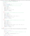 |
Figure A2 Matlab/GNU Octave computer code for sampling from a non-Gaussian distribution. |
Appendix: B KDE approximation of a PDF
If a Monte Carlo simulation is performed for a model with univariate data saved in a text file Omega.txt then a Kernel Density Estimate (KDE) algorithm may be implemented to approximate the Probability Density Function (PDF) as shown in Figure B1 using the Python Seaborn statistical library and the matplotlib graphical routine.
 |
Fig. B1 Python computer code for implementing a KDE approximation of a PDF. |
References
- S. Kline, F. Mcclintock, Describing uncertainties in single-sample experiments, Mech. Eng. 75, 3–8 (1953) [Google Scholar]
- BIPM, IEC, IFCC, ILAC, ISO, IUPAP, and OIML, “Evaluationof measurement data - Guide to the expression of uncertainty in measurement, ” tech. rep., JCGM/WG1 GUM, 2008. Revised 1st edition − https://www.bipm.org/en/publications/guides/https://www.bipm.org/en/publications/guides/. [Google Scholar]
- V. Ramnath, Determining the covariance matrix for a nonlinear implicit multivariate measurement equation uncertainty analysis, Int. J. Metrol. Qual. Eng. 13, 1–15 (2022) [CrossRef] [EDP Sciences] [Google Scholar]
- P. Kang, C. Koo, H. Roh, Reversed inverse regression for the univariate linear calibration and its statistical properties derived using a new methodology, Int. J. Metrol. Qual. Eng. 8, 1–10 (2017) [CrossRef] [EDP Sciences] [Google Scholar]
- V. Ramnath, Comparison of straight line curve fit approaches for determining variances and covariances, Int. J. Metrol. Qual. Eng. 11, 16pp (2020) [CrossRef] [EDP Sciences] [Google Scholar]
- Q. Tang, Q. Yang, X. Wang, A.B. Forbes, Pointing error compensation of electro-optical detection systems using Gaussian process regression, Int. J. Metrol. Qual. Eng. 12, 1–6 (2021) [Google Scholar]
- N. Habibi, A. Jalid, A. Salih, H. Hanane, Estimation of parallelism measurement uncertainty according to the geometrical product specifications standard using coordinate measuring machine, Int. J. Metrol. Qual. Eng. 14, 1–7 (2023) [CrossRef] [EDP Sciences] [Google Scholar]
- N. Habibi, A. Jalid, A. Salih, M.Z. Es-sadek, Perpendicularity assessment and uncertainty estimation using coordinate measuring machine, Int. J. Metrol. Qual. Eng. 14, 1–13 (2023) [CrossRef] [EDP Sciences] [Google Scholar]
- G.L. Bretthorst, The maximum entropy method of moments and bayesian probability theory, AIP Conf. Proc. 1553, 3–15 (2013) [CrossRef] [Google Scholar]
- J. Kohout, Four-parameter Weibull distribution with lower and upper limits applicable in reliability studies and materials testing, Mathematics 11, 1–23 (2023) [Google Scholar]
- L. Ziyu, F. Yongling, Z. Shicheng, W. Jinkun, Study on rolling bearing life based on Weibull distribution and correlation coefficient optimization and maximum likelihood estimation, J. Phys.: Conf. Ser. 2383, 1–9 (2022) [Google Scholar]
- A. Rezaei, A.R. Nejad, Effect of wind speed distribution and site assessment on pitch bearing loads and life, J. Phys.: Conf. Ser. 2507, 1–9 (2023) [Google Scholar]
- A. Possolo, C. Merkatas, O. Bodnar, Asymmetrical uncertainties, Metrologia 56, 1–9 (2019) [Google Scholar]
- A.B. Forbes, Approaches to evaluating measurement uncertainty, Int. J. Metrol. Qual. Eng. 3, 71–77 (2012) [CrossRef] [EDP Sciences] [Google Scholar]
- T. Burr, S. Croft, B.C. Reed, Least-squares fitting with errors in the response and predictor, Int. J. Metrol. Qual. Eng. 3, 117–123 (2012) [CrossRef] [EDP Sciences] [Google Scholar]
- K.F. Wallis, The two-piece normal, binomial, or double Gaussian distribution: its origin and rediscoveries, Stat. Sci. 29, 106–112 (2014) [Google Scholar]
- M. Villani. R. Larsson, The multivariate split normal distribution and asymmetric principal components analyis, Commun. Stat. − Theory Methods 35, 1123–1140 (2006) [CrossRef] [Google Scholar]
- A. Azzalini, A. Capitanio, Statistical applications of the multivariate skew-normal distribution, J. Royal Stat. Soc. Ser. B 61, 579–602 (1999) [CrossRef] [Google Scholar]
- A. Azzalini, sn: The skew-normal and related distributions such as the skew-t, tech. rep., CRAN, 2019. https://cran.r-project.org/web/packages/sn/index.html. [Google Scholar]
- A. Ara, F. Louzada, The multivariate alpha skew Gaussian distribution, Bull. Braz. Math. Soc.: New Series 50, 823–843 (2019) [CrossRef] [Google Scholar]
- R. Willink, Representating Monte Carlo output distributions for transfereability in uncertainty analysis: modelling with quantile functions, Metrologia 46, 154–166 (2009) [CrossRef] [Google Scholar]
- E. Acar, M. Rais-Rohani, C.D. Eamon, Reliability estimation using univariate dimension reduction and extended generalised lambda distribution, Int. J. Reliab. Saf. 4, 166–187 (2010) [CrossRef] [Google Scholar]
- C.G. Corlu, M. Meterelliyoz, Estimating the parameters of the generalized lambda distribution: Which method performs best? Commun. Stat. Simul. Comput. 45, 2276–2296 (2015) [Google Scholar]
- S. Noorian, M.N. Ahmadabadi, The use of the extended generalized lambda distribution for controlling the statistical process in individual measurements, Stat. Optim. Inf. Comput. 6, 536–546 (2018) [CrossRef] [Google Scholar]
- B. Wang, fitgbd: Fit extended generalized lambda distribution (EGLD/GBD), tech. rep., CRAN, 2019. https://cran.r-project.org/web/packages/gb/index.html [Google Scholar]
- S. Su, M. Maechler, J. Karvanen, R. King, B. Dean, Fitting single and mixture of generalised lambda distributions (GLDEX), 2022. https://cran.r-project.org/web/packages/GLDEX/index. html [Google Scholar]
- G. Muraleedharan, C.G. Soares, C. Lucas, Characteristic and moment generating functions of generalised extreme value distribution (GEV), in Sea Level Rise, Coastal Engineering, Shorelines and Tides, edited by L.L. Wright (Nova Science Publishers, Inc., 2009), ch. 13, 1–9 [Google Scholar]
- H. Klakattawi, D. Alsulami, M.A. Elaal, S. Dey, L. Baharith, A new generalized family of distributions based on combining Marshal-Olkin transformation with T-X family, PLoS ONE 17, e0263673 (2022) [Google Scholar]
- A. Possolo, Copulas for uncertainty analysis, Metrologia 47, 262–271 (2010) [CrossRef] [Google Scholar]
- J. Segers, M. Sibuya, H. Tsukahara, The empirical beta copula, J. Multivariate Anal. 155, 35–51 (2017) [CrossRef] [Google Scholar]
- L. Lu, S. Ghosh, Nonparametric estimation of multivariate copula using empirical Bayes methods, Mathematics 11, 4383 (2023) [Google Scholar]
- V. Ramnath, Numerical analysis of the accuracy of bivariate quantile distributions utilizing copulas compared to the GUM supplement 2 for oil pressure balance uncertainties, Int. J. Metrol. Qual. Eng. 8, 1–29 (2017) [CrossRef] [EDP Sciences] [Google Scholar]
- P.M. Harris, C.E. Matthews, M.G. Cox, Summarizing the output of a Monte Carlo method for uncertainty evaluation, Metrologia 51, 243–252 (2014) [Google Scholar]
- P.M. Harris, M.G. Cox, On a Monte Carlo method for measurement uncertainty evaluation and its implementation, Metrologia 51, S176–S182 (2014) [Google Scholar]
- I. Smith, Y. Luo, D. Hutzschenreuter, The storage within digital calibration certificates of uncertainty information obtained using a Monte Carlo method, Metrology 2, 33–45 (2022) [CrossRef] [Google Scholar]
- N. Armstrong, G.J. Sutton, D.B. Hibbert, Estimating probability density functions using a combined maximum entropy moments and bayesian method. theory and numerical examples, Metrologia 1–15 (2019) [Google Scholar]
- T.A. O'Brien, K. Kashinath, N.R. Cavanaugh, W.D. Collins, J.P. O'Brien, A fast and objective multidimensional kernel density estimation method: fastKDE, Comput. Stat. Data Anal. 101, 148–160 (2016) [CrossRef] [Google Scholar]
- V. Ramnath, Analysis of approximations of GUM supplement 2 based non-Gaussian PDFs of measurement models with Rosenblatt Gaussian transformation mappings, Int. J. Metrol. Qual. Eng. 11, 1–16 (2020) [CrossRef] [EDP Sciences] [Google Scholar]
- M.H. Khanjanpour, A.A. Javadi, Experimental and CFD analysis of impact of surface roughness on hydrodynamic performance of a Darrieus hydro (DH) turbine, Energies 13, 1–18 (2020) [Google Scholar]
- M. Kadivar, D. Tormey, G. McGranaghan, A review on turbulent flow over rough surfaces: fundamentals and theories, Int. J. Thermofluids 10, 100077 (2021) [CrossRef] [Google Scholar]
- C.F. Colebrook, Turbulent flow pipe particular reference to the transition region between the smooth and rough pipe law, J. Inst. Civil Eng. 11, 133–156 (1939) [CrossRef] [Google Scholar]
- T. Adams, C. Grant, H. Watson, A simple algorithm to relate measured surface roughness to equivalent sand grain roughness, Int. J. Mech. Eng. Mechatr. 1, 66–71 (2012) [Google Scholar]
- M.A. Shockling, J.J. Allen, A.J. Smits, Roughness effects in turbulent pipe flow, J. Fluid Mech. 564, 267–285 (2006) [CrossRef] [Google Scholar]
- F.R. Hama, Boundary-layer characteristics for smooth and rough surfaces, Trans Soc. Naval Archit. Mar. Engrs 62, 333–358 (1954) [Google Scholar]
- M.V. Zagarola, A.J. Smits, Mean-flow scaling of turbulent pipe flow, J. Fluid Mech. 373, 33–79 (1998) [CrossRef] [Google Scholar]
- S.E. Haaland, Simple and explicit formulas for the friction factor in turbulent pipe flow, J. Fluids Eng. 105, 89–90 (1983) [CrossRef] [Google Scholar]
- R.W. Jeppson, Steady flow analysis of pipe networks: an instructional manual, tech. rep., Utah State University, Utah Water Research Laboratory, January 1974. Paper 300. [Google Scholar]
- B.J. McKeon, M.V. Zagarola, A.J. Smits, A new friction factor relationship for fully developed pipe flow, J. Fluid Mech. 538, 429–443 (2005) [CrossRef] [Google Scholar]
- J.J. Allen, M.A. Shockling, G.J. Kunkel, A.J. Smits, Turbulent flow in smooth and rough pipes, Phil. Trans. R. Soc. A 365, 699–714 (2007) [CrossRef] [PubMed] [Google Scholar]
- N. Afzal, Friction factor directly from transitional roughness in a turbulent pipe flow, J. Fluids Eng. 129, 1255–1267 (2007) [CrossRef] [Google Scholar]
- Y. Wang, R.Li, l. Luo, L. Ruan, Analysis of metrological characteristics of elbow flowmeter under rotating state, Int. J. Metrol. Qual. Eng. 12, 1–9 (2021) [Google Scholar]
- D.A. Gace, On the performance of a coriolis mass flowmeter (CMF): experimental measurement and FSI simulation, Int. J. Metrol. Qual. Eng. 13, 1–15 (2021) [Google Scholar]
- U.Y. Akcadag, G.S. Sariyerli, New apparatus for the determination of liquid density at primary level in TUBITAK UME, Int. J. Metrol. Qual. Eng. 13, 1–6 (2022) [CrossRef] [EDP Sciences] [Google Scholar]
- BIPM, IEC, IFCC, ILAC, ISO, IUPAP, OIML, Evaluation of measurement data − Supplement 1 to the Guide to the expression of uncertainty in measurement − Propogation of distributions using a Monte Carlo method, tech. rep., JCGM/WG1 GUM Supplement 1, 2008. 1st edition − https://www.bipm.org/en/publications/guides/https://www.bipm.org/en/publications/guides/ [Google Scholar]
- BIPM, IEC, IFCC, ILAC, ISO, IUPAP, OIML, Evaluation of measurement data − Supplement 2 to the Guide to the expression of uncertainty in measurement − Propogation of distributions using a Monte Carlo method, tech. rep., JCGM/WG1 GUM Supplement 2, 2011. 1st edition − https://www.bipm.org/en/publications/guides/https://www.bipm.org/en/publications/guides/ [Google Scholar]
- V. Ramnath, Application of quantile functions for the analysis and comparison of gas pressure balance uncertainties, Int. J. Metrol. Qual. Eng., 8, p. 4 (18pp) D (2017) [CrossRef] [EDP Sciences] [Google Scholar]
- M.G. Cox, The evaluation of key comparison data, Metrologia 39, 589–595 (2002) [Google Scholar]
- R. Willink, On revision of the guide to the expression of uncertainty in measurement: proofs of fundamental errors in Bayesian approaches, Measurement: Sensors 24, 100416 (2022) [CrossRef] [Google Scholar]
- R.T. Clemen, R.L. Winkler, Combining probability distributions from experts in risk analysis, Risk Anal. 19, 187–203 (1999) [Google Scholar]
- L.R. Mead, N. Papanicolaou, Maximum entropy in the problem of moments, J. Math. Phys. 25, 2404–2417 (1984) [CrossRef] [Google Scholar]
- R.A. Jahdali, S. Kortas, M. Shaikh, L. Dalcin, M. Parsani, Evaluation of next generation high order compressible fluid dynamic solver on cloud computing for complex industrial flows, Array 17, 1–17 (2023) [Google Scholar]
- V. Ramnath, Analysis and comparison of hyper-ellipsoidal and smallest coverage regions for multivariate Monte Carlo measurement uncertainty analysis simulation datasets, MAPAN-J. Metrol. Soc. India 1–16 (2019) [Google Scholar]
- L.I. Langelandsvik, G.J. Kunkel, A.J. Smits, Flow in a commercial steel pipe, J. Fluid Mech. 595, 323–339 (2008) [CrossRef] [Google Scholar]
- T.P. Hill, Conflations of probability distributions, Trans. Am. Math. Soc. 363, 3351–3372 (2011) [CrossRef] [Google Scholar]
- A.N. Spiess, C. Feig, C. Ritz, Highly accurate sigmoidal fitting of real-time PCR data by introducing a parameter for asymmetry, BMC Bioinform. 221, 1–12 (2008) [Google Scholar]
- P. Praks, and D. Brkic, Advanced iterative procedures for solving the implicit Colebrook equation for fluid flow friction, Adv. Civil Eng. 5451034, 1–18 (2018) [CrossRef] [Google Scholar]
- R.L. Burden, J.D. Faires, Numerical Analysis, 7th ed. (Brookes/Cole, 2001) [Google Scholar]
- E. Friedrich, D. Kretzinger, Vulnerability of wastewater infrastructure of coastal cities to sea level rise: a South African case study, Water SA 38, 755–764 (2012) [CrossRef] [Google Scholar]
- S. Chen, Optimal bandwidth selection for kernel density functionals estimation, J. Probab. Stat. 2015, 242683, 1–21 (2015) [CrossRef] [Google Scholar]
- S.-T. Chiu, Bandwidth selection for kernel density estimation, Ann. Statist. 19, 1883–1905 (1991) [Google Scholar]
- R. Chartrand, Numerical differentiation of noisy, nonsmooth data, ISRN Appl. Math. 11, 1–11 (2011) [CrossRef] [Google Scholar]
- E.L. Kosarev, E. Pantos, Optimal smoothing of noisy data by fast Fourier transform, J. Phys. E.: Sci Instru. 16, 537–543 (1983) [CrossRef] [Google Scholar]
- G. von Winckel, Matlab central file exchange # 4540, Legendre–Gauss quadrature weights and nodes, 2023. https://www.mathworks.com/matlabcentral/fileexchange/4540-legendre-gauss-quadrature-weights-and-nodes [Google Scholar]
- I. Bogaert, Iteration-free computation of Gauss-Legendre quadrature nodes and weights, SIAM J. Sci. Comput. 36, A1008–A1026 (2014) [Google Scholar]
Cite this article as: Vishal Ramnath, Application of maximum statistical entropy in formulating a non-gaussian probability density function in flow uncertainty analysis with prior measurement knowledge, Int. J. Metrol. Qual. Eng. 15, 6 (2024)
All Tables
Summary of proposed discretization scheme accuracies for sampling from a non-Gaussian PDF.
Representative engineering pipe flow specifications for a typical petroleum refinery.
All Figures
|
Fig. 1 Geometry of pipe inner wall surface roughness measurements scheme illustrating positive amplitudes in peaks and negative amplitudes in valleys in Nikuradse equivalent grain size diameter experiments. |
| In the text | |
|
Fig. 2 PDFs of the inner wall surface roughness for commercial grade steel pipes reported by Shockling et al. [43] and Langelandsvik et al. [63]. |
| In the text | |
|
Fig. 3 Comparison of equivalent PDFs of the peak and valley amplitudes reported by Shockling et al. [43] and Langelandsvik et al. [63]. |
| In the text | |
|
Fig. 4 Comparison of CDFs of the surface roughness amplitudes with noise. |
| In the text | |
|
Fig. 5 Surface roughness CDFs showing Savitzky-Golay filtering to avoid spurious maxima and minima. |
| In the text | |
|
Fig. 6 Illustration of multiple peaks producing a multiple root search for a non-Gaussian PDF statistical sampling. |
| In the text | |
|
Fig. 7 Illustration of procedure converting a nonmonotonic curve into a sequence of monotonic curves. |
| In the text | |
|
Fig. 8 Graphical summary of the convergence characteristics of the numerical sampling schemes. |
| In the text | |
|
Fig. 9 Illustration of a sequence of Colebrook equations with varying random roughness values. |
| In the text | |
|
Fig. 10 Empirical cumulative distributions of pipe friction factor for Shockley and Langelandsvik datasets. |
| In the text | |
|
Fig. 11 Probability density function curves for Shockley and Langelandsvik input data-sets on the Monte Carlo simulation outputs for the pipe friction factor λ values showing Gaussian, piecewise linear fit of peaks locations/relative values and kernel density estimate to the actual non-Gaussian probability density function. |
| In the text | |
|
Fig. 12 Final simulation results for the probability density function of the pipe friction factor using the maximum statistical entropy method with results for the Shockling and Langelandsvik non-Gaussian surface roughness data-sets. |
| In the text | |
|
Fig. 13 Flowchart summary of main steps to implement a MaxEnt refinement of a non-Gaussian PDF. |
| In the text | |
|
Figure A1 Python computer code for sampling from a non-Gaussian distribution. |
| In the text | |
|
Figure A2 Matlab/GNU Octave computer code for sampling from a non-Gaussian distribution. |
| In the text | |
|
Fig. B1 Python computer code for implementing a KDE approximation of a PDF. |
| In the text | |
Current usage metrics show cumulative count of Article Views (full-text article views including HTML views, PDF and ePub downloads, according to the available data) and Abstracts Views on Vision4Press platform.
Data correspond to usage on the plateform after 2015. The current usage metrics is available 48-96 hours after online publication and is updated daily on week days.
Initial download of the metrics may take a while.