| Issue |
Int. J. Metrol. Qual. Eng.
Volume 17, 2026
|
|
|---|---|---|
| Article Number | 8 | |
| Number of page(s) | 12 | |
| DOI | https://doi.org/10.1051/ijmqe/2026001 | |
| Published online | 06 May 2026 | |
Research article
Quantifying carbon emissions: Scope 1 (direct), 2 (indirect), and 3 (life-cycle)
National Physical Laboratory, Teddington, UK
* Corresponding author: This email address is being protected from spambots. You need JavaScript enabled to view it.
Received:
7
July
2025
Accepted:
21
January
2026
Abstract
We analyse carbon emissions of Scopes 1, 2, 3 and discuss several case studies to illustrate direct and indirect emissions using state-of-the art measurement science. Direct emissions (Scope 1) can be measured and modelled at the moment when they are created in the field, taking into account instrumental errors and uncertainties; indirect emissions (Scope 2) require complex modelling and quantification of uncertainties because of heterogeneous energy systems, incomplete information and lack of direct measurements in remote locations; value chain emissions (Scope 3) include estimates produced by the supply chain of the products whose total (direct, real-time indirect, and life-cycle) emissions are being estimated. As such, Scope 3 emissions represent the biggest challenge for modelling and uncertainty quantification, because some information may be missing temporarily (reducible errors) or inaccessible in principle (irreducible errors). Our study proposes a systematic approach to studying and reporting carbon emissions of the three scopes and offers a novel case study on Scope 2 emissions.
Key words: carbon emissions / emission scopes / measurements / standardization
© V. Livina et al., Published by EDP Sciences, 2026
 This is an Open Access article distributed under the terms of the Creative Commons Attribution License (https://creativecommons.org/licenses/by/4.0), which permits unrestricted use, distribution, and reproduction in any medium, provided the original work is properly cited.
1 Introduction
The Greenhouse Gas Protocol classifies greenhouse gas (GHG) emissions as three types or Scopes [1]. Scope 1 emissions are direct emissions from the sources where they can be directly measured using specialized equipment. Scope 2 emissions are indirect emissions from the use of power (electricity, heating and cooling). These emissions are almost instant in time, as energy is generated at the time of its consumption in some remote power plants, which often burn fossil fuels. Scope 3 emissions are all other indirect emissions due to the activities of a person or enterprise, including supply chain “from cradle to grave”, and these indirect emissions may be distributed in time, for months or longer, depending on the life cycle of a product or process.
There is a range of documents recently developed for quantification of carbon emissions by several standardization bodies: International Organization for Standardization (ISO), Comite Europeen de Normalization / Comite European de Normalization ‘Electrotechnique (CEN/CENELEC), British Standards Institution (BSI), Institute of Electrical and Electronics Engineers (IEEE), International Telecommunication Union (ITU), and others. For immediate practical purposes, the following standards can be applied to quantify Scope 1–3 emissions, as summarized in Figure 1.
Scope 1 emissions:
ISO 20181 Stationary source emissions. Quality assurance of automated measuring systems;
BS-EN 17255 Stationary source emissions. Data acquisition and handling systems - Specification of requirements for the installation and on-going quality assurance and quality control of data acquisition and handling systems;
BS-EN 15267 Air quality. Assessment of air quality monitoring equipment - Performance criteria and test procedures for stationary automated measuring systems for continuous monitoring of emissions from stationary sources.
Scope 2 emissions:
IEEE 1922 A Method to Calculate Near Real-Time Emissions of Information and Communication Technology Infrastructure;
ISO 30134-8:2022 Information technology - Data centers key performance indicators - Carbon usage effectiveness (CUE);
CEN TR18145 Environmentally Sustainable AI (published in March 2025);
IEEE P7100 Standard for Measurement of Environmental Impacts of Artificial Intelligence Systems (in preparation);
ISO DTR 20226 Information technology - Artificial intelligence - Environmental sustainability aspects of AI systems.
Scope 3 emissions:
ISO 5338 Information technology - Artificial intelligence - AI system life cycle processes;
ISO 14040 Environmental management - Life cycle assessment - Principles and framework;
ISO 14064-1 Specification with guidance at the organization level for quantification and reporting of greenhouse gas emissions and removals;
ISO 59020 Circular economy - Measuring and assessing circularity performance;
ITU L1410 Methodology for environmental life cycle assessments of information and communication technology goods, networks and services;
ITU L1480 Enabling the Net-Zero transition: Assessing how the use of information and communication technology solutions impact greenhouse gas emissions of other sectors.
All these standards can be obtained from the websites of the corresponding organizations, and the explicit web-links are omitted for simplicity.
 |
Fig. 1 Application of standards to quantify carbon emissions. |
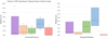 |
Fig. 2 Methane loss comparison. Left panel: summary box-whisker plots highlighting the range in methane emission factors (%) from indicated functional elements. Right panel: summary box-whisker plots highlighting the range in methane emission factors (%) from various functional elements for site which utilized agriculture feedstocks. Bars left to right with corresponding colours: purple - Digester, yellow - cogeneration system of heat and power (CHP), green - upgrade units, blue - digestate storage, orange - feedstock storage. |
2 Scope 1: direct emissions
To effectively work towards reducing greenhouse gas emissions derived from industrial processes and reach Net-Zero targets by 2050 [2], it is imperative that accurate and precise measurements of GHGs are conducted at their source. Carbon dioxide CO2 and methane CH4 are under particular scrutiny, in part due to their high radiative forcing effects and due to the prominence in being by-products of a large portion of industrial processes.
The vast majority of CO2 emitted to the atmosphere globally is derived from the combustion of hydrocarbons as fuel source for electricity production, see Figure 15 in [3]. Methane, however, can be released to the atmosphere as a byproduct of industrial processes such as landfill decomposition and enteric fermentation (Fig. 2). In addition to the direct release of GHGs, be it through stack emissions or by-product venting, a not inconsiderable quantity of emissions can be lost unintentionally via faults in the transmission and storage systems, as well as inadvertent venting through incomplete combustion. However, CH4 is not the only gas which can be emitted through fugitive emissions (i.e., undesirable industrial emissions due to leakage or discharge of gases and vapors). With the increasing prominence of carbon capture, utilization and storage of CO2 as a process to decarbonize many industrial processes, the storage and transmission of CO2 as a potential indirect source of emissions is becoming a factor in need of consideration. A comprehensive suite of measurement techniques is therefore required to tackle a host of emission sources and characteristics across many different industrial plants.
These emissions fall under the definition of Scope 1 emissions: direct emissions from sources which can be directly measured at their source using specialized equipment and methods. The measurement technique, or suite of techniques, implemented depend primarily on the type of emissions being released and the mechanisms of release (Fig. 3). However, the nature of the site, site operation methods and site dimensions can also play a part in the determination of which techniques are appropriate (Fig. 4). It should also be mentioned that some techniques are only valid for qualification of leaks in the form of detection, whilst others can be used for quantification. These various methods are also operated over different time scales, with them being categorized as either short-term or long-term.
It is important to note that there is currently no standardized vocabulary to describe the processes and monitoring of greenhouse gas emissions. Many reporting metrics for emissions can be used to describe a wide range of activities and characteristics. Some of them could be considered interchangeable, whereas others could be misleading if applied incorrectly. It is then crucial that a consistent framework of definitions and classifications of said processes and characteristics is determined. Such a framework was produced by the National Physical Laboratory (NPL) for use in methane monitoring methods and reporting requirements [4]. Frameworks like these improve the comparison of emissions inventories, while also facilitating data accessibility from numerous emission sources.
As mentioned previously, the majority of CO2 emissions are released due to the burning of fuel sources for electricity production. The regulations and legislation regarding reporting of CO2 emissions depends largely on the size of the industrial plant in question, as well as which industrial sector the site sits in. In Europe, under the Industrial Emissions Directive (IED), large combustion plants (LCPs) with thermal outputs greater than 50 MW have emission limit values (ELVs) dependent on the fuel source, thermal input and the type of combustion unit in use. Medium combustion plants (MCPs), with output <50 MWt and >1 MWt are under the Medium Combustion Plant Directive (MCPD), whilst combustion plants with output <1 MWt are under the regulatory power of local authorities. EU Emissions Trading Scheme (ETS) regulators are responsible for enforcing compliance of industries within the scope of this scheme.
For industries to be able to confidently ensure that they remain within these emissions limits, it is vital that they can accurately and to a certain degree of confidence measure the quantity of CO2 emitted within certain time frames. The processes by which this can be done, again, depend upon the size of the plant and the combustion fuel source. In the case of gas turbines in LCPs, due to the relatively simple chemical reaction of combustion, CO2 emissions can be calculated by multiplying emissions factors by the amount of fuel combusted or flow rate velocities. Due to the simplicity of this calculation, the resultant uncertainties are relatively low and fixed.
However, for more complex fuel sources this becomes more difficult, as with differing fuel sources it can become challenging to assume an emissions factor for the combustion activity. In these cases, direct measurements from in stack, point source measurements methods can provide a more realistic insight into a plant’s emissions profile. Operating under the EN14181 (ISO20181) quality assurance standard, e.g., monitoring waste-to-energy (WtE) combustion plants from in stack monitoring of flue gas can be taken directly from the emissions source using automated measuring systems (AMS, mainland Europe) or continuous emissions monitoring systems (CEMS, US & UK). The combustion of municipal-solid-waste (MSW) to generate energy for the grid is an increasing source of energy for many countries, whereby waste which would otherwise be disposed of in landfill is incinerated to generate a “greener” source of electricity. WtE plants are also under the jurisdiction of the IED.
Sites monitor their own emissions through CEMS and through the use of quality assurance levels (QALs). The sites are legally obligated to report AMS/CEMS values and it is assumed that the values reported are accurate.
To support that assumption, stationary source emissions sites are required to abide by several BS-EN standards; in particular BS-EN14181, BS-EN17255 and BS-EN15267. Through compliance with these standards and assessments such as QALs, emissions inventories can be derived. Due to the high number of parameters needing to be taken into consideration in this validation processes, and additional uncertainties derived from instrumentation, this form of emissions reporting results with larger uncertainties associated than those derived from emissions factors. Where direct monitoring data is unavailable, UNFCCC (United Nations Framework Convention on Climate Change) National Inventory Reports can be used as a source of GHG emissions data from a member state of the Paris Agreement.
Due to the more direct nature of CO2 emissions from combustion release to atmosphere, they are easier to monitor, regulate and measure. However, for more diffuse GHG emissions, this can be more challenging and as a result monitoring methods often accompany higher measurement uncertainties. Due to the non-direct causes of release, a suite of monitoring techniques can be used in conjunction to achieve a clearer picture of emissions profiles. The suitability of each method depends again on the size and scale of the emissions sources processes, the time-scales required, as well as the geometry of the sites.
Although not released in as large volumes as carbon dioxide, methane has a more severe global warming potential (GWP) in the short term, e.g., at the scale of 20 yr - see Table 8.7, page 714 [5]. In spite of this, the motivation behind the development of CH4 monitoring methods was initially an economic one, where industries aim to reduce loss of what is ultimately a commercial product through leaks. As the focus has shifted towards an environmental need to accurately measure unintended releases of methane for inventory reporting purposes, the measurement techniques have evolved as a result.
Differential absorption lidar (DIAL), tracer correlation (TC) and walk-over survey (comparable to leak detection and repair (LDAR) surveys within the oil and gas industry) campaigns have been utilized to monitor for such leaks. Within the Methane Emissions from Anaerobic Digestion (MEAD) project, DIAL, TC and walk-over surveys were used to detect and quantify leaks from anaerobic digestion (AD) facilities with gas-to-grid (GtG) capabilities [6,7].
The results of this research highlighted how the timing of such monitoring campaigns can impact the levels of emissions reported. The shorter-term monitoring methods such as those used in the MEAD project, act as a “snapshot” of measurements and offer only an insight into the emissions profile of each particular site during the measurement campaigns. In the case of AD sites, the feedstock also had a large impact on the emissions levels recorded, as well as that particular functional elements (FE) within transport network pipework are responsible for a larger number of leaks than others. However, walk-over surveys are not as effective (information on total emissions and effort/time needed) as other methods. Large industrial sites, such as Liquid Natural Gas (LNG) sites, often have a large site footprint and many areas are inaccessible or too hazardous for traditional LDAR surveys. Refineries often have even larger footprints than LNG sites and also have hazardous and inaccessible areas, however LDAR surveys are done regularly.
In this instance, DIAL surveys can be used to great effect. Similarly to the MEAD study, the DIAL was used to assess methane emissions from LNG sites and used to determine which FEs or groups of FEs were responsible [8]. All the FEs were responsible for some emissions, yet the aim was to determine the emission factors of each FE (not which one emitted more).
For the previously mentioned methods, unless standard operating procedures or emissions loss magnitudes are known, it is difficult to accurately assess as to whether the events recorded are one-off events or an insight into routine methane leakage. Operating procedures and data on operational status are well known and recorded by the operators, particularly for refineries and LNG sites. In the referenced work, the main scope was in effect to record operational data to derive EFs based on throughput (activity data). One of the conclusions was that one-off events were captured as well as emissions associated to particular operations. These short-term events would have been more difficult to detect (if not impossible) by Fugitive emission detection system (FEDS). The challenge for “snapshot” methodologies is to measure emissions under all operational procedures (particularly if there are many modes) and to capture the (long-term) variability in the emission that might well exist for constant operational mode. Essentially, the emission sources can be variable even under the same operating procedure (over the course of days, weeks, months) and this is when real-time measurements are needed to capture such variability.
FEDS can be used to cover longer time-scales, as “real-time” hourly-average concentrations, and can therefore give a better understanding of emission variability (both temporal and spatial) over time or during specific site operations and maintenance in ways which the short-term methods cannot, see the emissions webpage of NPL. The methodology by which ‘snapshot’ measurements are made/repeated might allow to capture information on variability.
As we move into an increasingly decarbonized world, methodologies originally implemented for the purpose of methane detection and quantification, are now being adopted for CO2 within CCUS (Carbon Capture, Utilization, and Storage) applications. DIAL research campaigns have also proven their applicability for measurement of CO2 from venting, overcoming the difficulties arising from high background atmospheric levels [9]. Development of walk-over surveys at component level for CO2 are ongoing, hoping to demonstrate the transferability of the methodologies across the two-emission source. Fugitive releases of CO2 will become an increasingly important area in need of monitoring as the globe moves towards Net-Zero, and further assessment of these methods are required.
While on the surface Scope 1 emissions appear to be the least challenging in terms of reporting, there are some caveats to this assumption. CO2 emissions from LCPs, taken directly from CEMS or through emissions factor calculations, whose compliance is regularly assessed through routine quality assurance procedures are considered the gold standard. However, it is appreciated that this is not always attainable, either due to technological limitations or time and financial restraints.
In light of this, the use of incentives which promote compliance to regulations where not necessary through legislation can be a way in which the sector moves towards better understanding of emissions release profiles, as well as better understanding of the uncertainties associated with the reported emission values. For comprehensive analysis of the sources of Scope 1 emissions to take place methodological monitoring techniques can be used alone or in parallel. Monitoring campaigns, aside from the primary role of reporting emissions, can identify FE which are routinely responsible for most emissions at sites and allow for proper processes, such as maintenance and repair schedules, to be put in place to help mitigate leaks, or indicate the need for abatement systems in stacks. However, issues with identifying and quantifying the uncertainty contributions of each measurement technique has proven difficult, and further study in the form of a comprehensive uncertainty analysis is needed.
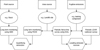 |
Fig. 3 Schematic depicting how emissions source type determines which monitoring methods are appropriate and the ultimate goal of each method. |
 |
Fig. 4 Schematic depicting how accessibility and spatial level dictates the monitoring methods used for fugitive emissions and the overlap in technologies which can be implemented. |
3 Scope 2: indirect emissions due to electricity use
Every industrial, urban or domestic activity requires supply of energy. When generated, electricity produces carbon emissions at the point of generation, and thus every electricity consumption process produces indirect (i.e., remotely generated) carbon emissions. These are called Scope 2 emissions. It is easy to estimate electricity consumption using electricity meters. With deployment of smart meters, with highly accurate measurements and known measurement uncertainty, it becomes possible to estimate Scope 2 carbon emissions from electricity use in real time.
In some European countries, such as France, the predominant source of energy generation is provided by nuclear power plants. In other European countries the fuel used may be more complex, including non-green fossil fuels with high carbon footprint, such as brown coal. With the deployment of renewable energy sources, the complexity and intermittency of multiple types of electricity generation must be considered. The fuel mix used for energy generation in Europe is particularly complex.
The UK National Grid currently reports the British fuel mix with a 5 min temporal resolution. The impact of cross-boundary European interconnectors (for example, from France to the UK) deliver electricity from other countries with different fuel mixes, and for Scope 2 emissions estimates these also need to be considered, along with the associated uncertainties on fuel types to obtain a combined uncertainty of the operational indirect carbon emissions from the power supply used by customers.
The Elexon portal of the National Grid provides open-access near real-time reports of fuel mixes in the national energy generation (the access to the publicly available data can be done via a registered profile in the Insights Real-Time Information Service, IRIS). Based on the known carbon factors of fossil fuels, as well as the interconnectors from the continent (for which average carbon footprints are known), it is possible to obtain the variable carbon intensity of the UK electricity grid, as shown in Figure 5. Such data can be used for estimation of the total footprint of the energy use, according to the power of the appliances, duration of use, taking into account reported uncertainties on fuels and equipment. In the recently developed CEN Technical Report “Environmentally Sustainable AI” this approach was applied for assessment of the carbon footprint of AI modelling (from development to training and deployment). This is particularly important in the context of ESG (Environmental, Social, Governance) reporting that is becoming mandatory for businesses across all industry sectors. Currently, such reporting is performed using averaged annual carbon factors, as it is done by the Department for Environment, Food and Rural Affairs (Defra) in the UK. However, the real dynamic carbon factor based on high-resolution (e.g., 30 min) fuel mix is noticeably different.
Using the dynamic carbon factor, we present a novel case study of Scope 2 carbon emissions for a large company (anonymized). Using the metered data and corresponding dynamical grid carbon intensity, we derived their carbon emissions as 967 plus-minus 48 tonnes over the period of three months (quarter one of the year 2024). We then repeated the analysis for six such quarters and summarized the results in Figure 6. In all of the quarters, the actual carbon emissions based on the real-time fuel mix and dynamical grid carbon factor were smaller than those estimated with a single annual factor value.
Because the UK grid carbon intensity is systematically decreasing due to planned decarbonization, the carbon factor announced in the beginning of the year, on average, is higher than actual carbon emissions, and this approach provides more accurate and smaller carbon emissions estimates, see Figure 6.
This case study illustrates the standardized methodology for estimation of indirect emissions due to electricity use, which is defined in the European standard CEN TR 18145 published in March 2025 under leadership of NPL [10].
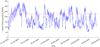 |
Fig. 5 UK grid carbon intensity obtained from the fuel mix reported by the National Grid with 30-min resolution, first quarter of the year 2024. The red dashed line denotes the annual Defra carbon factor that is used by companies for ESG reporting. |
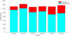 |
Fig. 6 Comparison of aggregated quarterly carbon emissions of a large company based on annual Defra carbon factors (dark red bars) and actual fuel-mix-based carbon factor of the UK National Grid (light cyan bars with uncertainty bars). |
4 Scope 3 emissions: life-cycle assessment
Scope 3 GHG emissions include life-cycle assessment (LCA), which is a method of analyzing the economic, environmental and social effects of a product throughout its entire life [11]. A variety of methods of LCA exist, often scoping different time periods of product's lifespan or displaying different structures of analysis.
The three main types for LCAs are cradle-to-grave, cradle-to-gate and cradle-to-cradle:
Cradle-to-grave is a full LCA from manufacture to disposal. It details all inputs and outputs for all phases of life, such the initial mining / acquisition of the materials, the emission output from transportation etc. This gives a holistic review of the impacts of the product in its entirety.
Cradle-to-gate is an assessment of product life cycle from manufacture to the factory gate (i.e., before transporting to the consumer). These assessments are often the basis for Environmental Product Declarations and usually omit the use and disposal phases.
Cradle-to-cradle is a specific kind of cradle-to-grave assessment where end-of-life (EOL) disposal step for the product is a recycling process. This process can yield new, identical products or different products [12].
Other LCA types include Life Cycle Energy Analysis (LCEA) and Well-to-Wheel:
Life cycle energy analysis accounts for all energy inputs, including energy to produce components, materials and services needed for the manufacturing process.
Well-to-wheel is an LCA type specifically used in reference to fuel use, tracing from raw material extraction to the use phase.
With the growing emphasis on environmental impact reduction in recent years, LCAs are pivotal within the production process. Their development allows for well-informed decision making across all business elements, as well as providing methods for comparison between different options for use within the business. Specifically, regarding lithium-ion batteries (LIBs), comparison between electric vehicles (EVs) and internal combustion engine vehicles (ICEs) would be irrelevant when comparing only use-phase emissions. To compare these, an entire cradle-to-grave LCA can be used to more accurately map the environmental and economical proficiencies and deficiencies of both engine types, returning more accurate results [13].
There are several legislative documents outlining frameworks and guidelines for life cycle analyses. In 1997, the ISO14040 standard was developed, and then the ISO14040 series standards were continuously published [14]. The ISO14040 series describes the principles and framework for LCA methods: namely, the definition of the goal and scope phase, life cycle inventory (LCI) phase, life cycle impact analysis (LCIA) phase and life cycle interpretation phase. ISO14040:2006 can be summarized in Figure 7, following [14].
According to the ISO14040 (Principles & framework) and ISO14044 (Requirements & Guidelines) of environmental management, there are two main types of impact category: midpoint and endpoint.
Midpoint methods examine environmental impacts earlier on the cause-effect chain before the endpoint is reached and are focused on single ecological problems.
Endpoint methods examine environmental impacts at the end of the cause-effect chain, and their indicators show environmental impacts at higher aggregation levels [13].
Publication [15] contains various protocols and standards, addressing the accountancy and reporting of corporate inventories with respect to greenhouse gas emissions. Separate protocols are put in place to address the nuances related to each emission scope. World Resources Institute also provides tools to aid the calculation of emissions. It discusses the types of uncertainty, where these can be found and how the GHG Protocol Uncertainty Tool accounts and quantifies these. Figure 8 demonstrates the process for estimating and aggregating parameter uncertainties for GHG inventories. The use of this tool and these guidelines allow the quantification of uncertainties within the calculations of some impact categories. This means more reliable measurements can be produced and more accurate conclusions can be drawn.
There are nationally determined contributions (NDC) that are targets for specific years, which are recognized internationally by UNFCCC. In the UK the Climate Change Committee (CCC) provide an independent recommendation for the NDC and carbon budgets, based on an achievable pathway of measures, allowing the Government to set appropriate targets and legislation to meet them.
Reliability in these measurements can allow businesses to work with greater confidence that they are abiding by these regulations and to prove their compliance if necessary. The accuracy of GHG measurements is crucial, especially in the UK, following the Climate Change Act [16] and Net-Zero Strategy [2]. This specifies carbon budgets, which are caps on UK carbon emissions, used as stepping-stones to get to the Net-Zero target goal in 2050. The carbon budgets are assessed as the average of emissions over a 5 yr period.
The European Commission recognizes LCAs as the best framework for assessing the potential environmental impacts of products currently available. They use the ISO14040 guidelines as the international standard and have used the method in multiple EU sanctioned projects [17]. In publication [18], the authors also note that the energy mix is important to aid the calculation of these factors. The LCI includes data collection and calculation procedures to quantify relevant inputs and outputs in the assessed system. Data collected can be separated into primary data (collected directly from the producers and users of the system) and secondary data (derived from the existing literature, including databases), see [13]. Data is then processed, often by specific LCA software.
An essential part of LCA is logging, which includes detailed description of the stages of development and used resources for development of a product. LCA logging requires reporting of each stage of energy supply (fuel mining, transportation, combustion (Scope 1 or 2 emissions, depending on the selected type of estimate), and disposal of the energy production waste. Currently, there is a CEN NWIP document at early stage of development on LCA logging that will systematically summarize this. In particular, it will include development of energy LCA ontologies and the ways of reporting them along the supply chain. A promising way to do this in a transparent and robust way is to employ blockchain open-source technologies.
Publication [19] recommends the use of representative primary data wherever possible, filling in gaps with secondary data which is validated by a third party and subject to only direct emissions calculations. Primary data should be collected on an annual basis, however, this may be too slow for some quickly changing industries, such as energy production. The rulebook then gives example data collection tables, designed to map out all the data needing to be collected for an accurate, representative LCA in the production and manufacturing stage.
Overall, primary data is more suitable for use, since the information and certainty around its capture is known, and the relevance of the data to the specific process is certain (e.g., the energy measurements taken from a primary generator can be used to calculate accurately the energy required to create an LIB, and the precise emissions attached. Energy mix would not need to be considered). The use of software tools will probably aid the structuring and completeness of LCAs. However, this is not a necessity; an accurate LCA can be structured and created without the use of specialist software. All studies found there had a lack of reliable primary data, meaning data was often extrapolated or manipulated from secondary to fill the gaps. One method of establishing how to reduce uncertainty is sensitivity analysis.
The authors of [13] found only eight studies that incorporate sensitivity analysis into their evaluations. These analyses can be organized using three main categories:
The first group is primarily concerned with energy mix consumed in production and use phases. A high percentage of non-renewables in these mixtures can significantly affect the end results of studies.
The second group refers to overall distance travelled by EVs in the battery's lifetime. It is important to consider different distances to improve robustness of the results.
The third group is concerned with the materials used in battery mechanisms and their recycling rates through (EOL) phases. This can help identify the elements with higher ecological influences and if rehabilitation methods generate more impacts than disposal [20].
Publication [18] discussed the use of sensitivity analyses to evaluate many options in the production phase, such as alternative mining processes. It also highlights the benefits of using sensitivity analyses to aid the evaluation of environmental impact categories and recommends all future studies to incorporate sensitivity analyses.
Publication [21] found 51% of papers conducted sensitivity analyses on their respective methods. However, many reviewed papers did not provide numerical values of the environmental impacts, and this complicates the comparison of results. Publication [19] states that sensitivity analyses should be carried out when using secondary data to calculate GHG emissions but does not delve into how those should be carried out.
There are factors to support both cradle-to-grave and cradle-to-gate analyses. The cradle-to-gate analyses can be more comparable, since use-cases are not specified and so processes are much more uniform. However, especially when considering the use case of EVs, use-phase analysis is required for an accurate LCA. [20] states that the use stage data must be modelled, possibly through primary data and assessing the energy flow of the reuse of electric vehicle batteries. Publication [13] concurs with this reasoning since the emission-saving benefits of EVs as opposed to ICEs occur mainly in the use phase. Furthermore, EOL stage documentation can be crucial for stakeholders and policymakers to make informed decisions for strategic development.
Further analysis can also be conducted within the EOL phases of the LCA. The two most common recycling methods are the cut-off and the substitution method [19]. The cut-off approach involves using recycled materials without credits or burdens, which means scrap input is burden free, but recycling material is credit free also. The substitution approach states that an amount of recycled secondary material will substitute an equivalent amount of primary material, which means credit is given to the substitution, but burdens are assigned to the scrap as an input.
In general, the cut-off approach is recommended since it is more transparent. However, both methods involve little consideration for material degradation and there is no guarantee that materials recycled will be a 1:1 replacement of primary materials.
Further studies are required to accurately evaluate the degradation of material over time. Furthermore, the repurposing of individual elements for lower intensity use-cases (e.g., using cobalt from batteries to make sensors) could be researched further, to find more effective and easy-to-implement uses [22]. It is also highlighted that blending cut-off and substitution recycling methods can lead to confusion and inconsistencies. For example, crediting for avoided burden by replacing primary materials in combination with recycling can lead to under-estimation of environmental impacts. Therefore, [22] recommends exercising caution when blending these methods.
Methods of impact category calculation are specified by the respective source methods. For example, impact categories for ReCiPe are described in [23] alongside their specific methods of calculation. Many of these calculations are “black boxes” for the user, meaning they simply input their data and return a result. However, most output values from general impact category calculations do not return a quantitative uncertainty.
For development of lithium batteries, usually the supply route is from East-Asian regions. Their supply chain may often be untraceable, especially at the stage of mining and transportation [24]. In terms of traceability, localized national mining represents the easier case of life-cycle assessment, as it makes it possible to trace the costs and resources within the national domain, using local legislation and shorter supply chain. Such an example in the UK is the company “Cornish Lithium” [25], which is investigating the opportunity for low-carbon production of lithium and other battery metals across Cornwall.
The locally operating company dedicated to sustainability and green targets may provide the basis for fully traceable life-cycle assessment of lithium batteries manufacturing, starting from mining lithium in the UK in hard rock and in geothermal waters, with full transparency and traceability.
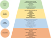 |
Fig. 7 Life cycle assessment categories following ISO 14040:2006. |
5 Gaps in carbon emissions assessment
In this section, we discuss the gaps in the assessment, in particular, in uncertainty quantification. We follow [26] in discussing reducible and irreducible uncertainties: those associated with unknowable things are irreducible, whereas uncertainties associated with knowable things that are currently unknown are reducible.
5.1 Scope 1
Scope 1 emissions and related uncertainties can be quantified using [27], i.e., by considering a measurement model through which the measurement uncertainty can be propagated. Bayesian techniques can be used for this purpose, and thus obtained uncertainties can be quantified. The choice of measurement model can help reduce errors, and we state that most of such errors are reducible, assuming high accuracy and suitable calibration of instruments. As such, Scope 1 carbon emissions that are measured in the field with high-quality instruments represent the case that can be addressed with conventional controlled techniques for uncertainty quantification.
There is a gap behind the assumption of high accuracy of calibrated instruments, as was mentioned earlier. Those estimates that are being done by technologies/methodologies (rather than by instruments) have the main limitation of lacking reliable verification to follow the deployment of the equipment/sensors, carrying out measurements and assessing uncertainties.
5.2 Scope 2
There is a challenge of uncertainty quantification of fuel mix for Scope 2 emissions: the calorific values of fossil fuels may vary significantly due to their natural variability, but what type and quality of the fuel that might be used at any given moment for electricity generation may not be possible to assess accurately. Thus, the uncertainty ranges of specific fuels may be inaccurate, which would influence uncertainty of the fuel mix. Coals and oils vary in their content; natural gas is predominantly methane but may have impurities and higher hydrocarbons. Because such fuel information can be retrieved from the national operator, this uncertainty is reducible if the full fuel information is provided. However, in practice, obtaining this information may be cumbersome and less likely to happen; rather an uncertainty range would be used from scientific literature, as was illustrated in the Scope 2 case study.
5.3 Scope 3
Scope 3 emissions represent the most complex case of uncertainty quantification, with some errors being currently irreducible. The main reason for that is the supply of materials and supply of parts over international supply chains. Therefore, it makes sense to distinguish two broad LCA cases: international and domestic. For domestic LCA analyses, it is possible to introduce blockchain techniques [28] for the full traceability of the parts and materials. Such examples already exist in the EU in the so-called short food supply chains [29], and some supermarkets report this in their promotional publications.
Both national and international supply chains may suffer lack of traceability, which depends on proper documentation and digitalization of each supply stage. For example, if transportation is outsourced to a less transparent company, or if some stage is split between several suppliers due to cost reduction, this may represent an obstacle for traceability. International supply chains may have additional issues due to translations between languages. However, with proliferation of digitalization, ML/AI tools for documentation processing, this is expected to improve, thus representing a reducible uncertainty.
6 Conclusion
The paper overviews the three scopes of carbon emissions and presents a novel case study on Scope 2 emissions. It also outlines the gaps in the three scopes and the metrological approach to their uncertainty quantification. While estimation of carbon emissions of Scopes 1 & 2 has metrologically robust approaches, in the area of GHG sensitivity analysis for life cycle assessment, no universal framework exists. This is likely because the nature of data (distribution of primary/secondary usage) and methods differ between studies, meaning that the assumptions and dimensions of input data vary.
Another cause for uncertainties within the LCAs analyzed is the inclusion and effect of energy mix. This is often due to the lack of precise information available, especially in secondary data sources (such as using geographical averages). A life cycle energy analysis could be used to more appropriately calculate these energies, however the time required to produce an LCEA alongside an LCA would be significant. UK National Grid maintains a public portal with fuel mix for energy generation reported at 5-min temporal resolution, which is useful for LCA at the national scale [30].
Despite the increasing use of LCAs in the study LIBs, the overall proportion of studies carried out in the industry remains very small. The increased research into LCA frameworks is a step in the right direction to allow comparable analyses. However, financial burdens and a lack of data remain the dominant causes for inaccurate and vague LCAs.
It is likely that in the foreseeable future (until mid-2030s) LIB technology will be the dominant battery technology in electric vehicles. The recent developments in sodium-ion batteries will likely allow for some, more niche, uses but the range of these batteries is not large enough for vehicle usage currently. Furthermore, it is likely to take at least 10 yr for solid-state battery technology to be sufficiently developed and researched that it can be more widely used in EVs [31].
EVs with solid state batteries are likely to start being rolled out in the next 2-3 years (Nissan – 2028 https://www.nissan-global.com/EN/INNOVATION/TECHNOLOGY/ARCHIVE/ASSB/ ; Toyota – 2027/28 https://www.toyota-europe.com/news/2023/battery-technology; BYD – from 2027 https://electrek.co/2026/02/09/byd-hits-solid-state-ev-battery-milestone-due-out-as-soon-as-2027/) with wider adoption from 2030, i.e. 5 years rather than 10. This paper from 2024 suggests at least 5 years (https://doi.org/10.1016/j.sctalk.2024.100382), so maybe replace that as [31] and change it to 5 years rather than 10.
It is reasonable to start with a localized case study based fully in the UK, starting from mining lithium for battery manufacturing to battery decomposition and waste utilization in the UK. This will provide a traceable case study with a fully controlled and documented supply chain. Single-country analysis, with support of national legislation, provides reliable ground for a metrologically robust analysis. In other countries, a solution could be to create a software framework which logs all business energy certificates and usage to aid both emission and impact category calculations.
Overall, the areas where metrological specialists could have the most impact are in the frameworks set-up to allow businesses to supply their data accurately and systematically, be that in a blockchain database, such that companies can publish their results without risk of engaging competition or be that in sensitivity analysis such that assumptions made can be more accurately accounted for. The intention of these additions is that companies could carry out their LCAs at a cheaper cost and therefore, would be more inclined to carry them out. This would provide more data to analyses and make conclusions more accurate, but only if the data is of a decent quality. This could lead to more development and research being carried out to improve efficiency and decrease negative impacts.
Acknowledgments
The authors are grateful to Spencer Thomas (HSES NPL) for support in analyzing Scope 2 carbon emissions.
Funding
This work was funded by the UK Government's Department for Science, Innovation & Technology through the UK's National Measurement System programmes.
Conflicts of interest
The authors declare that they have no known competing financial interests or personal relationships that could have appeared to influence the work reported in this paper.
Data availability statement
Due to the proprietary nature of the data, it cannot be made openly available. The data can be made available from the corresponding author upon reasonable request, subject to a non-disclosure agreement. Contact the lead author for further information.
Author contribution statement
All authors equally contributed to discussion, development, writing, and reviewing of the paper.
References
- Greenhouse Gas Protocol, https://ghgprotocol.org [Google Scholar]
- Net Zero Strategy: Build Back Greener, 2021, https://www.gov.uk/government/publications/net-zero-strategy [Google Scholar]
- International Energy Agency, CO2 Emissions in 2023, https://www.iea.org/reports/co2-emissions-in-2023 [Google Scholar]
- A. Connor, J. Shaw, A framework for classifying methane monitoring requirements, emission sources and monitoring methods, NPL Report ENV 52, (2024), https://doi.org/10.47120/npl.ENV52 [Google Scholar]
- Climate Change, The physical science basis, in: T.F. Stocker, D. Qin, G.-K. Plattner, M. Tignor, S.K. Allen, J. Boschung, A. Nauels, Y. Xia, V. Bex, P.M. Midgley (Eds.), Contribution of Working Group I to the Fifth Assessment. Report of the Intergovernmental Panel on Climate Change, Cambridge University Press, Cambridge, United Kingdom and New York, NY, USA, 2013, 1535 pp. https://www.ipcc.ch/site/assets/uploads/2018/02/WG1AR5\_all\_final.pdf [Google Scholar]
- N. Howes, F. Innocenti, A. Finlayson, C. Dimopoulos, R. Robinson, T. Gardiner, Remote measurements of industrial CO2 emissions using ground-based differential absorption lidar in the wavelength region, Remote Sensing, 15, 1–21 (2023) [Google Scholar]
- N. Howes, F. Innocenti, A. Finlayson, J. Shaw, J. Connolly, L. Nguyen, Methane from Anaerobic Digestion (MEAD) Study, NPL Report, 2023 [Google Scholar]
- F. Innocenti, R. Robinson, T. Gardiner, N. Howes, N. Yarrow, Comparative assessment of methane emissions from onshore LNG facilities measured using differential absorption lidar, Environ. Sci. Technol. 57, 3301–3310 (2023) [Google Scholar]
- DIAL for Remote Emissions Measurement, NPL 2018, https://www.npl.co.uk/getattachment/products-services/Environmental/Absorption-Lidar-DIAL/instruments-dial-flyer.pdf?lang=en-GB [Google Scholar]
- CEN DTR 18145 Environmentally Sustainable AI, March 2025 [Google Scholar]
- S. Farjana, Introduction to life cycle assessment, Chapter 1. Life Cycle Assessment for Sustainable Mining, 1–13 (2021) [Google Scholar]
- I. Muralikrishna et al, Chapter five - life cycle assessment, Environ. Manag. 57–75 (2017) [Google Scholar]
- A. Temporelli, M. Carvalho, P. Girardi, Life cycle assessment of electric vehicle batteries: an overview of recent literature, MDPI: Energies, 13, (2020) [Google Scholar]
- X. Lai et al., Critical review of life cycle assessment of Lithium-ion batteries for electric vehicles: a lifespan perspective, eTransportation, 12, 100169 (2022) [Google Scholar]
- World Resources Institute, A corporate accounting and reporting standard (The Green House Gas Protocol, 2015), https://ghgprotocol.org/calculation-tools, https://ghgprotocol.org/sites/default/files/Global-Warming-Potential-Values, https://ghgprotocol.org/sites/default/files/ghg-uncertainty.pdf [Google Scholar]
- Climate Change Act, Climate Change Act, 2008. https://www.legislation.gov.uk/ukpga/2008/27/contents [Google Scholar]
- European Commission, European Platform on Life Cycle Assessment (LCA), 2023, https://ec.europa.eu/environment/ipp/lca.htm [Google Scholar]
- J. Porzio et al., Life-cycle assessment considerations for batteries and battery materials, Adv. Energy Mater. (2021) [Google Scholar]
- Global battery alliance, Greenhouse gas rulebook (GBA, 2022) [Google Scholar]
- F. Arshad, Life cycle assessment of lithium-ion batteries: a critical review, Resour. Conserv. Recycl. 180, 106164 (2022) [Google Scholar]
- R. Tolomeo, G. De Feo, R. Adami, L. Sesti Osso, Application of life cycle assessment to lithium ion batteries in the automotive sector. MDPI: Sustainability, 12, (2020) [Google Scholar]
- A. Nordelof, S. Poulikidou, M. Chordia, F. Bitencourt de Oliveira, J. Tivander, R. Arvidsson, Methodological approaches to end-of-life modelling in life cycle assessments of lithium-ion batteries, MDPI Batteries, 5, (2019) [Google Scholar]
- M. Huijbregts et al., ReCiPe 2016. National Institute for Public Health and the Environment, (2016) [Google Scholar]
- L. Zeng, S. Liu, E. Kozan, P. Corry, M. Masoud, A comprehensive interdisciplinary review of mine supply chain management, Resour. Policy 74, 102274 (2021) [Google Scholar]
- Cornish Lithium (https://cornishlithium.com/projects/), Sustainability Report https://cdn.sanity.io/files/rui0grfj/production/89dfad955515ebbdd452d47f2276daae1559430d.pdf [Google Scholar]
- A. Der Kiureghian, Measures of structural safety under imperfect states of knowledge, J. Struct. Eng. 115, (1988), UC Berkley. [Google Scholar]
- JCGM 100:2008 Evaluation of measurement data - Guide to the expression of uncertainty in measurement, 2008, https://www.bipm.org/documents/20126/2071204/JCGM100-2008E.pdf [Google Scholar]
- A.L.C. Merlo, D.S. Mendonca, J. Santos et al., Blockchain for the carbon market: a literature review, Discov. Environ. 3, 68 (2025) [Google Scholar]
- EIP-AGRI Focus Group: Innovative Short Food Supply Chain Management, 2015, https://ec.europa.eu/eip/agriculture/sites/default/files/eip-agri_fg_innovative_food_supply_chain_management_final_report_2015_en.pdf [Google Scholar]
- Insights Real-Time Information Service (IRIS), https://bmrs.elexon.co.uk/iris [Google Scholar]
- D. Finegan, M. Scheel, J. Robinson, B. Tjaden, I. Hunt, T. Mason, J. Millichamp, M. Michiel, G. Offer, G. Hinds, D. Brett, P. Shearing, In-operando high-speed tomography of lithium-ion batteries during thermal runaway, Nat. Commun. 6, 6924 (2015) [Google Scholar]
Cite this article as: Valerie Livina, Hannah Cheales-Norman, Marc Coleman, Tom Gardiner, Jack Clarke, Thomas Smith, Neil Howes, Rod Robinson, Quantifying carbon emissions: Scope 1 (direct), 2 (indirect), and 3 (life-cycle), Int. J. Metrol. Qual. Eng. 17, 8 (2026), https://doi.org/10.1051/ijmqe/2026001
All Figures
|
Fig. 1 Application of standards to quantify carbon emissions. |
| In the text | |
|
Fig. 2 Methane loss comparison. Left panel: summary box-whisker plots highlighting the range in methane emission factors (%) from indicated functional elements. Right panel: summary box-whisker plots highlighting the range in methane emission factors (%) from various functional elements for site which utilized agriculture feedstocks. Bars left to right with corresponding colours: purple - Digester, yellow - cogeneration system of heat and power (CHP), green - upgrade units, blue - digestate storage, orange - feedstock storage. |
| In the text | |
|
Fig. 3 Schematic depicting how emissions source type determines which monitoring methods are appropriate and the ultimate goal of each method. |
| In the text | |
|
Fig. 4 Schematic depicting how accessibility and spatial level dictates the monitoring methods used for fugitive emissions and the overlap in technologies which can be implemented. |
| In the text | |
|
Fig. 5 UK grid carbon intensity obtained from the fuel mix reported by the National Grid with 30-min resolution, first quarter of the year 2024. The red dashed line denotes the annual Defra carbon factor that is used by companies for ESG reporting. |
| In the text | |
|
Fig. 6 Comparison of aggregated quarterly carbon emissions of a large company based on annual Defra carbon factors (dark red bars) and actual fuel-mix-based carbon factor of the UK National Grid (light cyan bars with uncertainty bars). |
| In the text | |
|
Fig. 7 Life cycle assessment categories following ISO 14040:2006. |
| In the text | |
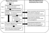 |
Fig. 8 Uncertainty quantification process, carried out by the GHG Protocol Uncertainty Tool [15]. |
| In the text | |
Current usage metrics show cumulative count of Article Views (full-text article views including HTML views, PDF and ePub downloads, according to the available data) and Abstracts Views on Vision4Press platform.
Data correspond to usage on the plateform after 2015. The current usage metrics is available 48-96 hours after online publication and is updated daily on week days.
Initial download of the metrics may take a while.