| Issue |
Int. J. Metrol. Qual. Eng.
Volume 16, 2025
|
|
|---|---|---|
| Article Number | 5 | |
| Number of page(s) | 10 | |
| DOI | https://doi.org/10.1051/ijmqe/2025004 | |
| Published online | 01 July 2025 | |
Research Article
Application of SIFT operator with binocular vision fusion in Building engineering measurement
Chongqing Metropolitan College of Science and Technology, Chongqing 402167, China
* Corresponding author: This email address is being protected from spambots. You need JavaScript enabled to view it.
Received:
7
May
2024
Accepted:
16
May
2025
Abstract
With the increasing demand for higher accuracy and reliability in the field of engineering measurement, traditional methods have shown a series of problems when facing complex scenarios and precision measurement tasks. Therefore, a scale invariant feature transformation engineering measurement method integrating binocular vision is proposed. This study focuses on binocular vision three-dimensional dimension measurement, using two-dimensional chessboard for monocular and binocular calibration to obtain internal and external reference information. At the same time, the scale invariant feature transformation algorithm has been simplified, combined with epipolar geometry to improve matching performance. The experiment showed that the improved scale invariant feature transformation algorithm achieved a matching accuracy of 97%. After fusing binocular vision, the close range matching was improved to 98%, the matching time was reduced to 1.8 seconds, and the number of feature points was reduced to 24. In distance measurement, the minimum error for planar targets was 0.25%, the maximum error for curved targets was 1.08%, and the overall maximum error percentage was 2.24%. The scale invariant feature transformation operator that integrates binocular vision has achieved significant results in engineering measurement, showing higher accuracy and reliability in three-dimensional dimension measurement compared to traditional methods. This innovative method is expected to improve measurement accuracy and reliability, providing a more accurate and feasible solution for three-dimensional dimension measurement in the engineering field.
Key words: binocular vision / scale invariant feature transformation / camera calibration / three dimensional measurement / engineering survey
© C. Li and R. Deng, Published by EDP Sciences, 2025
 This is an Open Access article distributed under the terms of the Creative Commons Attribution License (https://creativecommons.org/licenses/by/4.0), which permits unrestricted use, distribution, and reproduction in any medium, provided the original work is properly cited.
1 Introduction
The increasingly stringent demand for engineering surveying in modern society requires higher precision and comprehensive data acquisition and analysis for complex projects in fields such as architecture, civil engineering, and infrastructure monitoring [1]. However, traditional measurement methods are limited when facing challenges such as complex environments, changes in lighting, and target occlusion, and there is an urgent need for innovative technological means to improve the robustness and accuracy of measurements [2]. On the other hand, Scale Invariant Feature Transform (SIFT) is known for its invariance in scale, rotation, and brightness changes as an efficient and accurate measurement tool [3,4]. The binocular vision (BV) system can capture two slightly offset images of the same scene and obtain depth information of the scene, namely the 3D structure, thereby achieving more comprehensive and stereoscopic visual perception [5]. Based on this, this study proposes an engineering measurement method BV-SIFT that integrates BV and SIFT operators. This study conducted an in-depth analysis of camera imaging models and calibration methods, using 2D checkerboard calibration objects to locate targets on left and right cameras and obtain internal and external parameter information. In addition, a detailed analysis is conducted on the basic principles of the SIFT algorithm, including steps such as scale space generation, spatial point detection, key point direction determination, and feature descriptor generation. In view of the problems in matching efficiency and accuracy of the SIFT algorithm, this study proposes a simplified SIFT that combines epipolar geometry and Random Sample Consistency (RANSAC) algorithm, aiming to improve matching performance and make it more suitable for various needs in different scenarios. Through these key technological means, this study aims to optimize the BV measurement system and improve its accuracy and reliability in 3D dimension measurement. The innovation of this study is to achieve BV application using SIFT operator in engineering measurement by conducting in-depth research on camera calibration, SIFT algorithm optimization, and matching performance improvement.
This study is divided into five parts. Section 1 introduces the research background, problems, and solutions of engineering surveying. Section 2 provides an overview of the research achievements in engineering surveying, summarizing the difficulties and shortcomings of the methods. Section 3 introduces the design optimization method for the engineering measurement model of BV-SIFT. Section 4 designs performance verification tests to verify the effectiveness of the proposed BV-SIFT measurement method in practical engineering measurements. Section 5 summarizes the research methods, analyzes the experimental results, and proposes the shortcomings and prospects of the methods.
2 Related works
Engineering surveying, as a key branch of the engineering field, plays an important role in civil engineering, construction engineering, and infrastructure construction. Its demand for accurate acquisition and processing of spatial information is particularly significant in urbanization, infrastructure construction, and environmental monitoring. Many scholars have conducted a series of studies on it. Daun et al. used a mixed approach, combining quantitative and qualitative data, to explore the differences between practitioners' needs for technology transfer and the commonly proposed methods in academia. There was a mismatch between the demand for industry professionals and the commonly proposed technology transfer methods [6]. Bendory et al. proposed the use of auto-correlation analysis to estimate the rotation and translation invariant features of target images in low signal-to-noise ratio domains. It aimed to address the challenges in low signal-to-noise ratio environments in multi-object detection. Regardless of the noise level, this technique could be successfully used to recover target images from high noise measurement images when the measurement was sufficiently large [7]. Rodríguez-Alabanda et al. developed a software specifically designed, analyzed, and optimized for multi-step wire drawing industrial processes. This computer-aided manufacturing software had significant potential in promoting students' ability-based learning goals [8]. Kong and Song used the YOLOv3 network and K-means clustering method to select optimized clustering anchor boxes, aiming to cope with the complexity of urban traffic scenes. The average accuracy and recall of its object detection reached 84.49% and 97.18%, respectively, which is 7.76% and 4.89% higher than the original YOLOv3 [9].
The SIFT operator is a computer vision algorithm used to detect and describe local features in digital images. The advantage of the SIFT operator lies in its strong invariance and discrimination, making it excellent in image matching and object recognition in complex scenes. Karim et al. used feature extraction methods based on SIFT and Support Vector Machine for offline Arabic handwriting recognition, aiming to address the challenges of this recognition method. The proposed method achieved a recognition rate of 99.08%, demonstrating efficiency for handwritten Arabic words [10]. Prastasti designed an image recognition currency application based on the Android platform. This program used the SIFT method for feature extraction to obtain better accuracy from complex calculations, aiming to improve people's recognition accuracy of currency authenticity [11]. Zhao et al. proposed a fast unmanned aerial vehicle image stitching method based on SIFT, aiming to improve its stitching efficiency and effectiveness. This method has achieved significant improvement in crop growth monitoring [12]. Singh et al. proposed a robust image hashing technique to address the issue of easy manipulation of digital data. This method was superior to other existing technologies and provided an effective solution for authentication and recognition of digital images [13].
In summary, engineering surveying, as a key branch of the engineering field, is very important in civil engineering, construction engineering, and infrastructure construction. However, the current challenges faced by engineering surveying include data processing challenges in complex environments, balancing accuracy and efficiency, and robustness requirements for transformations such as scale and rotation. Moreover, the SIFT operator has scale invariance and rotation invariance, enabling it to robustly extract key feature points in images, thus having good adaptability to common image transformations in engineering measurements. Based on this, engineering measurement based on SIFT operator can solve the common data processing challenges in complex environments in engineering measurement. It provides important technical support for precise measurement and visualization in the engineering field.
3 BV engineering measurement technology based on SIFT operator
The research focuses on the key technical principles in binocular stereo vision (BSV), covering image acquisition, camera calibration, stereo calibration, image preprocessing, stereo matching, and 3D depth information acquisition. The research objective is to enable the engineering field to achieve functions such as image alignment, 3D point cloud reconstruction, automatic object detection, and multi image stitching by extracting SIFT feature points.
3.1 BSV engineering testing technology
The camera imaging model involves the relationship between images, cameras, and the world coordinate system. This model is a mathematical description of how a camera captures light and converts it into an image [14]. One of the most widely used models is the pinhole camera model. In this model, the image coordinate system is used to represent the pixel positions in the image. The camera coordinate system describes the internal parameters and relative positions of the camera. The world coordinate system represents the 3D space of the actual scene. Through the transformation relationships of these coordinate systems, this study is able to understand the process of camera imaging and perform accurate image processing and calculations. Figure 1 shows the pinhole model.
In the model shown in Figure 1, it is assumed that there is a small pinhole in front of the camera, through which light is projected onto the imaging plane, forming an inverted image [15]. This model is based on several assumptions, such as the straight propagation of light, the pinholes being very small to avoid scattering, and the refraction of light at the pinholes. In the absence of distortion, the mathematical relationship between image pixels and the physical coordinate system is equation (1).
 (1)
(1)
In equation (1), (u, v) represents a point in the pixel coordinate system of the image. u0 and v0 represent the physical dimensions of pixels in the u-axis and v-axis directions, which are dx and dy, respectively. The camera coordinate system is achieved through orthogonal rotation matrix R and 3D translation vector. T is converted from the world coordinate system, and the expression is equation (2).
 (2)
(2)
The physical coordinates of point (x, y) on the plane and the camera coordinate system are shown in equation (3).
 (3)
(3)
The BSV system is based on two cameras on the left and right capturing images from different angles of the same scene. This involves the relative position between two cameras, represented by the rotation matrix and translation vector [16]. This affects the common field of view for both cameras, affecting the search range for image matching and the determination of 3D coordinates for object feature points. Therefore, establishing an effective computer BSV system is crucial. The structure of a binocular stereo system is generally divided into head-up binocular structure (HBS) and non-head-up binocular structure (N-HBS) based on whether the optical axes of two cameras are parallel. The HBS of BSV is Figure 2.
In Figure 2, HBS refers to two cameras with parallel optical axes, simplifying image matching and making processing and algorithms more intuitive and efficient. It is commonly used for close range tasks such as object localization and ranging. However, for processing long-distance or large parallax scenes, their depth information may be limited. Through camera calibration, the internal and external parameters of the camera can be determined, thereby establishing an accurate camera model [17]. Camera calibration can correct the distortion caused by the camera lens and solve the problem of scale. This study used Zhang Zhengyou's calibration method, assuming that the equation of the template's plane in the world coordinate system is Z = 0 and the translation vector is r1, r2. For any point on a plane, the derived translation transformation relationship can be expressed as equation (4).
 (4)
(4)
In equation (4),  and
and  represent 3D and 2D points in the spatial plane.
  represents the camera projection formula. P represents the camera intrinsic matrix. R identifies the rotation matrix. T represents the translation vector. H is a homography matrix. Assuming the H matrix is written in the form of three column vectors, with a scaling factor λ, equation (5) can be obtained.
 (5)
(5)
In equation (5), r1 r2 are two orthogonal unit vectors. Images captured through binocular cameras are often affected by lighting, temperature, and other factors, and contain random noise and distortion [18]. To improve accuracy, it is necessary to preprocess the original image. The goal of preprocessing is to improve visual effects and facilitate computer processing, including contrast enhancement, edge feature enhancement, denoising, and pseudocolor processing.
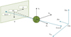 |
Fig. 1 Pinhole model. |
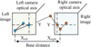 |
Fig. 2 Binocular stereovision horizontal binocular structure. |
3.2 Engineering image preprocessing and stereo matching technology
Image noise can be divided into two types: artificial and natural. The goal of image smoothing is to remove these noises, which can be performed in both spatial and frequency domains [19]. Neighborhood averaging is a commonly used spatial domain processing method that reduces noise by taking the average of eight pixels near the reference point, as shown in equation (6).
 (6)
(6)
In equation (6), f(x, y) represents the original image. S represents a domain selected for each pixel of f(x, y). g(x, y) represents the average pixel value of the corresponding image after smoothing. M represents the pixels in domain S. Median filtering is a typical nonlinear filtering technique that can solve the problem of image detail blur caused by linear filters under specific conditions. Its expression is equation (7).
 (7)
(7)
In equation (7), W represents a 2D template. Image blur is essentially caused by the influence of averaging or integration operations on the image. To enhance the edges of image contours, differential operations can be performed to make the image clearer. The commonly used image sharpening methods include gradient operators and Laplacian operations. In continuous variables (X) and (Y), for a 2D continuous function, its gradient at point (x, y) is defined as equation (8).
 (8)
(8)
In equation (8), f(x, y) is a continuous 2D function. For digital images, gradients are usually achieved through differentiation rather than strict differentiation. The expression for the first-order difference in the horizontal and vertical directions is equation (9).
 (9)
(9)
The SIFT feature point matching algorithm is based on the detection and description of key points. By detecting extreme points in an image and extracting scale space features from the surrounding area, it generates feature descriptors with scale invariance [20]. This algorithm mainly includes five steps: generating scale space (GSS), detecting and locating spatial points, determining the direction of key points, generating feature descriptors, and matching feature points. Among them, GSS is designed to simulate the multi-scale features of image data. The Gaussian Laplacian scale space definition of a 2D image is equation (10).
 (10)
(10)
In equation (10), (x, y) represents pixel coordinates, σ represents scale coordinates, and G(x, y, σ) represents a variable scale Gaussian function. The expression of the Gaussian function is equation (11).
 (11)
(11)
The SIFT algorithm introduces a pyramid structure to accelerate the speed of feature point extraction, and generates a gradually decreasing resolution Gaussian map through Gaussian smoothing and downsampling. The image pyramid contains O groups, each with S layers, and the values from O to S are set as needed. The schematic diagram of the scale space and the Difference of Gaussian (DOG) scale space is Figure 3.
In Figure 3, the scale space generates a series of gradually decreasing resolution images by performing multiple Gaussian convolutions on the images to simulate image features at different scales. And DOG highlights the changes in the image by calculating the differences between adjacent scale spatial layers. After determining the extreme points, low contrast and unstable points are removed, and then the key points are accurately located through 3D quadratic function fitting. Finally, the Taylor quadratic expansion of the scale space function DOG was used for least squares fitting. To take the derivative of the spatial scale function to be 0, and the exact position of the extremum point is obtained, as shown in equation (12).
 (12)
(12)
In equation (12),  represents the exact position of the extreme point. This study further utilizes image gradients to determine the direction of key points, obtains gradient direction distribution features by sampling neighboring pixels, and assigns directional parameters to each key point. To maintain the invariance of key points, a feature descriptor is generated for each key point. The SIFT feature algorithm uses multidimensional vectors to describe features and fully depict details. To maintain rotation invariance, the coordinate axis is first rotated to the direction of the feature point, and then an 8 × 8 image window is selected with that point as the center.
In Figure 4, the blue dots in the left image are feature points, and the surrounding 64 neighboring pixels are represented by small grids. Each grid has arrows representing the gradient direction, and the size of the arrows represents the gradient intensity. The blue circle represents the Gaussian weighted range, with pixels closer to the feature points having a greater impact. The image is divided into 4 × 4 small blocks, and the 8 directional gradient histograms of each block are counted to obtain 4 seed points, forming a feature point. This study further simplifies the SIFT algorithm, and Figure 5 shows the improved feature descriptors.
In Figure 5, the first 128 dimensional feature descriptor is simplified to 24 dimensions: by significantly reducing the number of feature points, the matching speed is improved. This is because generating 128 dimensional feature vector descriptors takes a long time, which affects the efficiency of the algorithm. By using a simplified operator method, after the initial matching, a secondary matching is performed by combining epipolar geometry and RANSAC algorithm. Mismatches in the initial matching are eliminated, further improving the matching accuracy. The gradient modulus and direction of pixels inside two circular rings are calculated, and the feature vectors of the two rings are normalized. After processing, the expression for the feature vector of the internal ring is equation (13).
 (13)
(13)
In equation (13), D represents the eigenvector of the inner ring. After the initial matching, the RANSAC algorithm is used to optimize the basic matrix and matching point pairs. This process first randomly selects some matching point pairs, calculates the basic matrix, then traverses all matching point pairs, and finally calculates the percentage of matching point pairs that satisfy the basic matrix model at a specific threshold. The above steps are repeated until the basic matrix with the maximum percentage is determined. To reconstruct 3D spatial points, it is necessary to find corresponding points in two images. Figure 6 shows the principle of polar geometry.
Figure 6 identifies point P1 in images I1 and I2, performs feature point matching, and finds the point P2 that best matches P1 in I2 according to specific criteria. The two are projections of the same world coordinate system point Pw. Usually, the midpoint Pl in the left image is determined first, and the corresponding point P2 in the right image is searched throughout the entire image. But this search method is time-consuming and may lead to incorrect matches. To solve this problem, the concept of epipolar constraint was introduced, which restricts the search path of corresponding points to a straight line. This study developed an image size detection software platform. In the process of 3D image size detection, the 3D image information is first obtained. In 3D space, to consider a point P(xw,yw,zw), whose projection points on the image plane are pl(xl, y) and pr(xr, y), respectively. According to the principle of similar triangles, the expression for depth Z can be derived, as shown in equation (14).
 (14)
(14)
Depth information Z represents the coordinate value zw of spatial point P in the world coordinate system. Assuming the parallax is d, where d = xl − xr, the coordinate value of the spatial 3D point P is represented as equation (15).
 (15)
(15)
This study further obtained a set of data by performing approximate regular cylinder analysis on the obtained 3D images, and achieved millimeter level accuracy through analysis and measurement. By fitting the 3D information of key points, the radius of the object can be restored. From this, it can be determined whether the measured object conforms to the cylindrical equation.
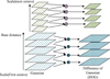 |
Fig. 3 Scale space and Do G scale space. |
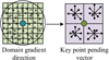 |
Fig. 4 Key point neighborhood ladder information generated descriptors. |
 |
Fig. 5 Modified characteristic descriptors. |
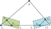 |
Fig. 6 Schematic diagram of polar geometry. |
4 Engineering measurement performance detection based on improved SIFT algorithm
This chapter aims to evaluate the performance and real-time performance of improved traditional SIFT algorithms. In the VS2012 simulation environment, this study used the open-source OpenCV library to program and simulate the improved SIFT algorithm, and conducted a series of SIFT feature point matching experiments to verify its real-time performance.
4.1 Defect detection based on YOLOv3 algorithm
Before the experiment begins, defect images must be captured in different lighting scenarios and angles, with a total of 3000 images collected to establish a dataset. Subsequently, a YOLOv3 training program was developed using Matlab, and parameters were optimized during the training process, with a total of 200 training rounds. The total loss value of YOLOv3 includes position, confidence, and classification error, and its loss function curve is Figure 7a. Furthermore, the accuracy curve was obtained through calculation, and the results are presented in Figure 7b.
Figure 7(a) shows the recall curve, where the loss value decreases before about 100 training iterations and gradually stabilizes after about 100 iterations. Figure 7b shows the average accuracy mean curve. Before about 20 training iterations, the accuracy curve loss value showed an upward trend, and gradually stabilized at around 40 training iterations.
Figure 8a shows the recall curve, and Figure 8b shows the average precision mean curve. Before about 30 training sessions, the loss values of the two curves showed an upward trend. When the training frequency is around 30 times, the loss value shows a sudden decrease trend, then increases again, and finally gradually stabilizes. The loss values of both curves exceed 0.9, and the maximum average accuracy is 83.28%.
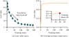 |
Fig. 7 Recall rate curve and average accuracy mean curve. |
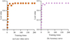 |
Fig. 8 Recall rate curve and average accuracy mean curve. |
4.2 Performance detection based on BV
This study conducted experiments using VS2008 based on the OpenCV library, selecting cylindrical engineering objects as matching objects and obtaining left and right images through a camera. Firstly, the SIFT algorithm was used to extract image features. Although most feature points were successfully detected, some mismatches were caused by insufficient lighting. The shadow part of the object generated feature descriptors, but the algorithm generated a large number of descriptors and matching pairs, resulting in poor performance. In contrast, the SURF algorithm performs better but still has mismatches. A simplified algorithm has been proposed for the SIFT problem, which reduces feature descriptors while improving matching accuracy and efficiency. Table 1 shows the matching results.
Table 1 shows the overall matching accuracy, matching time, and number of mismatches of the three algorithms. The proposed method has the highest matching accuracy, reaching 97%, with the lowest number of mismatches, only 1, and the overall performance is the best. By simplifying the SIFT operator and combining it with the RANSAC algorithm, a mismatched pair was successfully removed after the initial matching, retaining 24 pairs of inliers. The matching efficiency is between SIFT and SURF, suitable for scenarios with high matching accuracy and less strict real-time performance. The experimental data of the combination of SIFT and RANSAC for performing secondary matching after initial matching are shown in Table 2.
In Table 2, after integrating the BV method, the accuracy of close range matching reaches 98%, the matching time is only 1.8 seconds, a decrease of 0.5 seconds, and the feature points are reduced from 31 to 24. The accuracy of long-range matching has increased from 83% to 93%. This study further conducted target ranging experiments using the BV system, using an improved algorithm to calculate the distance between flat and circular objects at different distances, and compared and analyzed the results with the actual distance. For different types of obstacles, different methods were used to determine the target distance, and different range values were set for the distance between the baseline midpoint and the target object, and corresponding measurement data was collected. The distance measurement data (planar target) of the improved SIFT algorithm is Figure 9.
In Figure 9a, when the actual distances are 500 mm, 650 mm, and 700 mm, the measured distances of the targets are 502.86 mm, 635.43 mm, and 713.42 mm. In Figure 9b, it has errors of 2.86 mm, −14.57 mm, and 13.42 mm, with error percentages of 0.57%, 2.24%, and 1.91%. The distance measurement data (surface target) of the improved SIFT algorithm is shown in Figure 10.
In Figure 10a, when the actual distance is 500 mm or 700 mm, the measured distance of the target is 503.65 mm or 707.58 mm. When the actual distance is, the measured distance of the target is. In Figure 10b, it has errors of 3.65 mm and 7.58 mm, with error percentages of 0.73% and 1.08%. In summary, the maximum error percentage of the measurement algorithm is 1.08%.
Matching results.
Matching data of the two methods for different image environments.
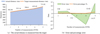 |
Fig. 9 Improved SIDET algorithm for distance measurement data (planar object). |
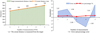 |
Fig. 10 Distance measurement data of improved SIET algorithm (curved object). |
5 Conclusion
To meet the demand for high precision and reliability in the field of engineering measurement, this study proposes a SIFT operator engineering measurement method that integrates BV. This study used the SIFT operator based method to perform monocular and binocular calibration on 2D chessboard grids, obtaining internal and external parameter information. Simplifying the SIFT algorithm by combining epipolar geometry and RANSAC algorithm has improved matching performance to meet different scene requirements. The experiment showed that the improved SIFT algorithm has achieved significant results in matching, with an accuracy rate of 97% and only one mismatch. After fusing BV, the close range matching rate increased to 98% and the matching time was shortened to 1.8 seconds. In terms of distance measurement, for a planar target, when the actual distance was 650 mm, there was an error of −14.57 mm, with an error percentage of 2.24%. When the actual distance of the curved target was 700 mm, the error was 7.58 mm, and the error percentage was 1.08%. In summary, the maximum error percentage of the measurement algorithm was 2.24%. The SIFT operator that integrates BV exhibited higher accuracy and reliability in 3D dimension measurement compared to traditional methods. Compared with the existing engineering measurement methods, such as the traditional SIFT algorithm, the proposed method here has a significant improvement in accuracy and efficiency. The method has a matching accuracy of 97% and the least number of mismatches. The improved SIFT algorithm combined with RANSAC achieved 98% close matching accuracy and long-range matching accuracy from 83% to 93%.
This innovative method is expected to improve measurement accuracy and reliability, providing a more accurate and feasible solution for 3D dimension measurement in the engineering field. Although there have been some achievements in stereo vision research this time, due to time and capability limitations, research on key technologies such as camera calibration and stereo matching is still not in-depth enough. However, there are still some limitations in the research. The research method depends on the hardware performance of the camera, which may introduce additional errors in practical applications. Therefore, in future research, the camera calibration errors can be compensated with inertial measurement units or sensor fusion to improve the calibration stability. HDR sensors can be used to solve the problem of uneven illumination, or multi-exposure image fusion technology can enhance feature extraction in low/high light environments.
Funding
The research is supported by 2021 “Measurement and valuation of installation engineering”, Chongqing Municipal first-class course, Chongqing Education High Letter (2021) No. 31.
Conflicts of interest
The authors declare no conflict of interests.
Data availability statement
All data generated or analysed during this study are included in this published article.
Author contribution statement
This study focuses on binocular vision three-dimensional dimension measurement, using two-dimensional chessboard for monocular and binocular calibration to obtain internal and external reference information. C. L. analyzed the data and R. D. helped with the constructive discussion. C. L. and R. D. made great contributions to manuscript preparation. All authors read and approved the final manuscript.
References
- P.K. Choudhury, Student assessment of quality of engineering education in India: evidence from a field survey, Qual. Assur. Educ. 27, 103–126 (2019) [CrossRef] [Google Scholar]
- G.W.T.C. Kandamby, The formative assessments for building drawings, Int. J. Civil Struct. Environ. Infrastruct. Eng. Res. Dev. 9, 51–60 (2019) [Google Scholar]
- S. Zhao, P. Wang, Q. Cao, H. Song, W. Li, Weakly supervised salient object detection based on image semantics, J. Comput. −Aided Des. Comput. Graph. 33, 270–277 (2021) [Google Scholar]
- K. Jang, Y.‐K. An, B. Kim, S. Cho, Automated crack evaluation of a high‐rise bridge pier using a ring‐type climbing robot, Comput. Aided Civil Infrastruct. Eng. 36, 14–29 (2021) [CrossRef] [Google Scholar]
- M. Ouziala, Y. Touati, S. Berrezouane, D. Benazzouz, B. Ouldbouamama, Optimized fault detection using bond graph in linear fractional transformation form, Proc. Inst. Mech. Eng. I 235, 1460–1471 (2021) [Google Scholar]
- M. Daun, J. Brings, P.A. Obe, An industry survey on approaches, success factors, and barriers for technology transfer in software engineering, Software: Pract. Exp. 53, 1496–1524 (2023) [CrossRef] [Google Scholar]
- T. Bendory, T.Y. Lan, N.F. Marshall, Multi-target detection with rotations, Inverse Probl. Imag. 17, 362–380 (2023) [CrossRef] [PubMed] [Google Scholar]
- O. Rodríguez-Alabanda, G. Guerrero-Vaca, P.E. Romero, L. Sevilla, Educational software tool based on the analytical methodology for design and technological analysis of multi‐step drawing processes, Comput. Appl. Eng. Educ. 27, 38–48 (2019) [CrossRef] [Google Scholar]
- F.F. Kong, B.B. Song, Improved YOLOv3 panoramic traffic monitoring target detection, Comput. Eng. Appl. 56, 20–25 (2020) [Google Scholar]
- A. Karim, S. Mahdi, A.A. Mohammed, Arabic handwriting word recognition based on scale invariant feature transform and support vector machine, Iraqi J. Sci. 60, 381–387 (2019) [Google Scholar]
- A.L. Prasasti, Design of foreign currency recognition application using scale invariant feature transform (SIFT) method based on android (case study: Singapore dollar), J. Eng. Appl. Sci. 14, 6991–6997 (2019) [CrossRef] [Google Scholar]
- J. Zhao, X. Zhang, C. Gao, Rapid mosaicking of unmanned aerial vehicle (UAV) images for crop growth monitoring using the SIFT algorithm, Remote Sens. 11, 1226–1227 (2019) [CrossRef] [Google Scholar]
- K.M. Singh, A. Neelima, T. Tuithung, Robust perceptual image hashing using SIFT and SVD, Curr. Sci. 117, 1340–1344 (2019) [CrossRef] [Google Scholar]
- M.E. Sahin, Image processing and machine learning‐based bone fracture detection and classification using X‐ray images, Int. J. Imag. Syst. Technol. 33, 853–865 (2023) [CrossRef] [Google Scholar]
- L. Sun, S. Qu, Y. Du, Bio-inspired vision and neuromorphic image processing using printable metal oxide photonic synapses, ACS Photon. 10, 242–252 (2023) [CrossRef] [Google Scholar]
- F. Jeon, M. Griffin, A. Almadori, Measuring differential volume using the subtraction tool for three-dimensional breast volumetry: a proof of concept study, Surg. Innov. 27, 659–668 (2020) [CrossRef] [PubMed] [Google Scholar]
- D.W. Becker, R. Knopp, F. Kunkel, Precision oncology revolutionizes nuclear medicine using a theranostic approach, Der Nuklearmediziner 42, 321–327 (2019) [CrossRef] [Google Scholar]
- D. Uhlig, M. Heizmann, Model-independent light field reconstruction using a generic camera calibration, TM-Technisches Messen 88, 361–373 (2021) [CrossRef] [Google Scholar]
- H. Mokayed, T.Z. Quan, L. Alkhaled, V. Sivakumar, Real-time human detection and counting system using deep learning computer vision techniques, Artif. Intell. Appl. 1, 221–229 (2023) [Google Scholar]
- P.P. Groumpos, A critical historic overview of artificial intelligence: issues, challenges, opportunities, and threats, Artif. Intell. Appl. 1, 197–213 (2023) [Google Scholar]
Cite this article as: Chune Li, Rui Deng, Application of SIFT operator with binocular vision fusion in Building engineering measurement, Int. J. Metrol. Qual. Eng. 16, 5 (2025), https://doi.org/10.1051/ijmqe/2025004
All Tables
All Figures
|
Fig. 1 Pinhole model. |
| In the text | |
|
Fig. 2 Binocular stereovision horizontal binocular structure. |
| In the text | |
|
Fig. 3 Scale space and Do G scale space. |
| In the text | |
|
Fig. 4 Key point neighborhood ladder information generated descriptors. |
| In the text | |
|
Fig. 5 Modified characteristic descriptors. |
| In the text | |
|
Fig. 6 Schematic diagram of polar geometry. |
| In the text | |
|
Fig. 7 Recall rate curve and average accuracy mean curve. |
| In the text | |
|
Fig. 8 Recall rate curve and average accuracy mean curve. |
| In the text | |
|
Fig. 9 Improved SIDET algorithm for distance measurement data (planar object). |
| In the text | |
|
Fig. 10 Distance measurement data of improved SIET algorithm (curved object). |
| In the text | |
Current usage metrics show cumulative count of Article Views (full-text article views including HTML views, PDF and ePub downloads, according to the available data) and Abstracts Views on Vision4Press platform.
Data correspond to usage on the plateform after 2015. The current usage metrics is available 48-96 hours after online publication and is updated daily on week days.
Initial download of the metrics may take a while.